Wednesday, September 25, 2019

Getting back to normal after a long summer

It has been a fun summer, sort of.

13 weeks ago, I had my left knee replaced to balance out my other two hip replacements on my right side. This is hopefully the last time that Dr Morrison of Southern Joint Replacement Institute ever has to cut into parts of my body with power tools. (Never say never, but all my other joints are in decent enough shape comparatively!) For this surgery I did something I did not do for my last two. I kind of shut out the SQL world for a while. I barely worked for 4 weeks, and I didn’t blog or pay attention to several book projects I am working on currently.

This was kind of a wonderful feeling, but I definitely started missing writing blogs, articles, and a book I had started working on with a group of authors earlier in the year. The book had to come first before I got back into the real world, and last Saturday night, I finished my parts that were of the critical path of getting it done. (I revised (fairly heavily) two chapters, then tech edited half of the book. So far, I am pretty proud of my time on the book, and I expect the output to be really great.

The book is “SQL Server 2019 Administration Inside Out”, from Microsoft Press. You can find out more about here.

It has even been a fairly long time between conferences for me too. My last SQL Saturday was SQL Saturday Chattanooga, where I was on the leadership team. I missed Louisville, where I had been to every one of the events prior, as well as a few others like Indianapolis that I had been to the prior year. It was kind of hard to watch from the Twitterverse this year, but it was kind of restful there too. I also worked on the crew for Music City Tech again this year, which was in early September.

My next SQL Saturday I have scheduled is SQL Saturday Memphis, cause you know, I gotta support my Tennessee folks! I will be doing my newest presentation, Relational Design Critique, which I really enjoy with a group. I put up a design, and we discuss the issues with the model. Later that week, I will travel out to Richmond to their user group and do the presentation for them (their group was actually the inspiration for the presentation, as something VERY similar was on their list of possible topics for the year!)

The next SQL Saturday I plan to submit to is Nashville (http://www.sqlsatnash.com), my second home! Tammy and Kerry do a great job, and I look forward to attending, and maybe speaking. 

If any of my other editors happen to read this, know that you (and only you) are the next up on my to do list. No one else but you. Not any other SQL project, not my Disney Picture a Day twitter feed, not my Dollywood Pictures twitter feed, not even planning for my upcoming trip to Disney World to see Galaxy’s Edge, and certainly not planning a SQL Saturday, Music City Tech, PASS Summit, or even time with my grandkids. Just you!

The post Getting back to normal after a long summer appeared first on Simple Talk.


from Simple Talk https://ift.tt/2myyuP7
via

Building Machine Learning Models to Solve Practical Problems

Machine learning has been reshaping our lives for quite a while now. Be it the smallest thing such as unlocking your phone through Face Recognition to useful interactions with Siri, Alexa, Cortana, or Google using Speech Recognition, machine learning is everywhere! In this article, I am going to provide a brief overview of machine learning and data science. With a basic understanding of these concepts, you can dive deeper into the details of linear regression and how you can build a machine learning model that will help you to solve many practical problems. The article will focus on building a Linear Regression model for Movie Budget data using various modules in Python. It will make use of prebuilt data science modules such as Pandas, Matplotlib and Scikit-learn to build an efficient model. First, I’ll start with a brief introduction about different terms in the data science and machine learning space, then move the focus to Python coding so that you can actually start building your own machine learning model.

Machine Learning

As the name indicates, making machines learn what humans can do is machine learning. It’s all about making computers and applications learn and become decisive without explicitly programming all the possibilities. Based on known data or various possibilities with correct answers provided to the algorithms, the computer should yield the solutions to a given problem when the answer is not known.

In my previous article, I gave a granular view of components involved in machine learning which might help you to get a conceptual understanding of how Data, Model and Algorithms are interconnected.

Data Science

At its heart, data science is about turning the data into value. Data science can be thought of as the application for finding certain patterns in data and through that pattern deduce the outcome for the future problem at hand. It’s a combination of data mining and computer science. Initially, data mining was done using statistics, but with the help of data science, it’s mainly done programmatically. The powerful programming languages such as Python and R provide support to various scientific computing packages that leverage building statistics-focused models to predict the solutions.

As the name suggests, data science is all about data. There are various steps involved from collecting the data to processing and analysing the data. At each step, the different actors/roles come into play as shown in the table below:

Steps Involved

Different Processes at each step

Roles

Collect Data

Data or content from various sources

Data Analyst

Move/Store Data

Structured and Unstructured Data Storage

Data Analyst

Clean/Explore/ Transform Data

Cleaning and ETL

Data Scientist

Aggregate/Label Data

Analytics, training and aggregate data

Data Scientist

Learn/Optimize Data

ML Algorithms, AI and A/B Testing

Machine Learning expert

Many data professionals, including DBAs and ETL developers, are familiar with most of these steps as well!

Linear Regression

Linear regression is the core concept in data science. It is a statistical term and mainly used whenever there is a need to make a prediction, model a phenomenon or discover the relationships between things. It is used for finding the relationship between two continuous variables. One of them is an independent variable, and the other is a dependent variable. Linear regression is used for determining the hypothesis. The core idea is to find the relationship between the two variables and obtaining a line that best fits the data. The best line is the one for which the most predictions are close to correct, which means the chances of errors are very low.

Here’s an example to help you understand linear regression. Assume that you are given the data for all the past movie productions: the movie budget and the revenue that they collected through the box office or any other sources. Now, imagine that you want to produce a movie and you want to predict from previous movie successes how much money your movie will make.

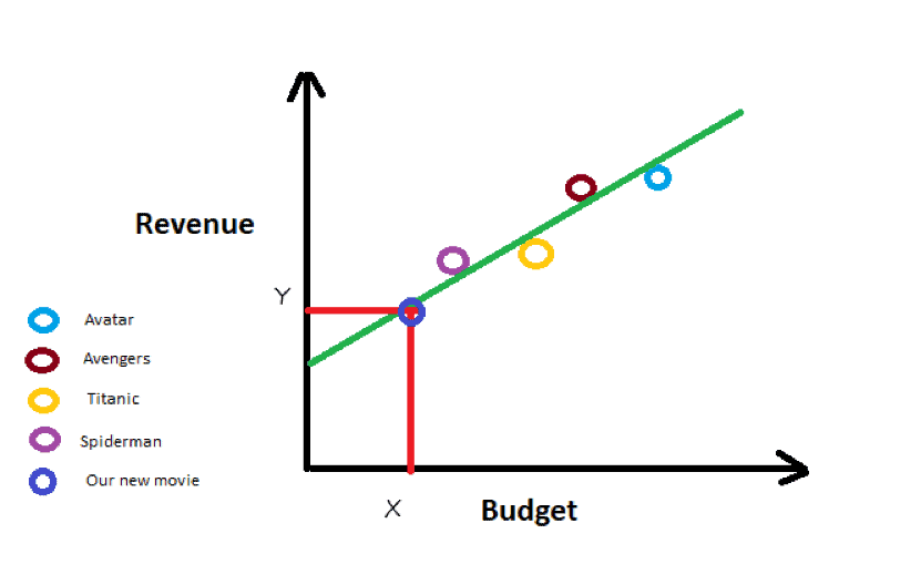
Given the data about various successful high budget films such as Avatar, Avengers, Titanic, etc., you can perform a hypothesis and try to understand where your movie fits. You are essentially going to build the best line (green line in the image below) that will help you predict how much revenue the movie can make given the budget of the film.

Through the budget value (X) for the movie, you can predict how much revenue (Y) the movie is going to make by just making a line from budget onto the best line (green line).

Requirements 

Many languages such as Python, R, and Scala, etc., provide support for data science by bringing together statistics, data analysis and their related strategies to understand and analyse the data. This article will show how to use Python to analyse the data. Python has long been known as an easy to learn programming language from a syntax point of view. It provides extensive support to statistical and data science related libraries such as NumPy, SciPy, Scikit-learn, and Keras, etc. It also has an active community with a vast selection of libraries and resources which makes Python as the first choice for many data scientists.

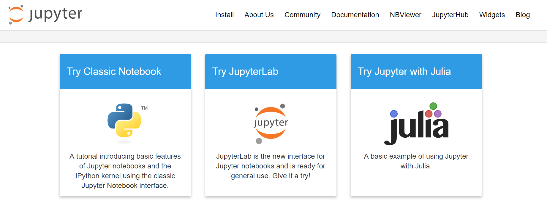
Jupyter Notebook is an incredible tool that provides an easy way to execute the Python code. This article will use the browser version of Jupyter Python Notebooks. Click on Try Classic Notebook after you go to this link.

Editor’s note: you can also use the Jupyter Notebook feature found in Azure Machine Learning Studio, Azure Data Studio, or Azure Machine Learning Services.

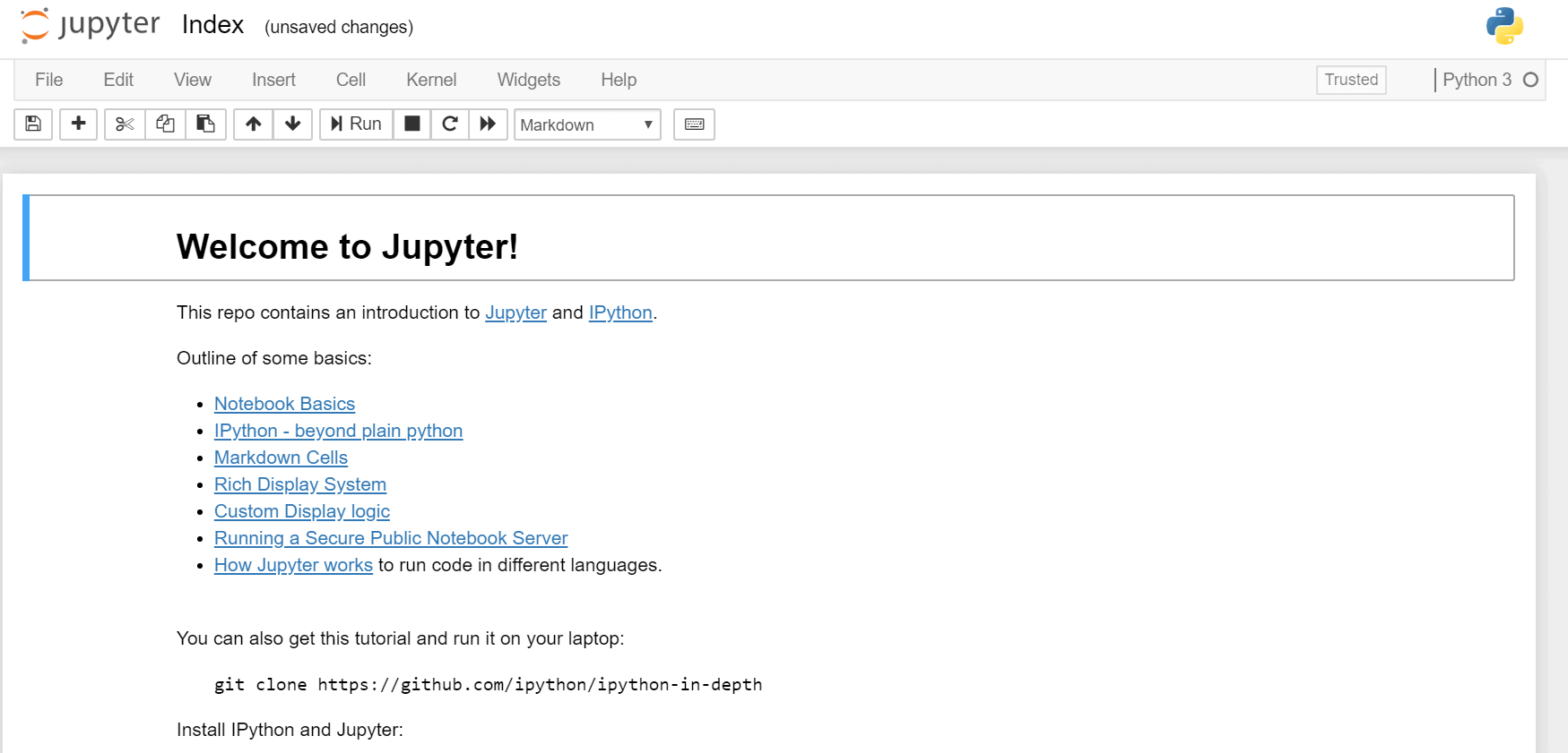
This will open a new Python notebook in the browser where you can write Python commands and see the results.

Note: The browser version of Jupyter Notebook sometimes gets disconnected if it is kept idle for a long time. You may try downloading Anaconda and after installation is complete open the Jupyter notebook. This will help you run the Jupyter notebook on the local computer without connectivity issues.

Before writing some interesting Python commands and cooking something, you need to gather and clean the ingredients for the recipe.

Start building the model

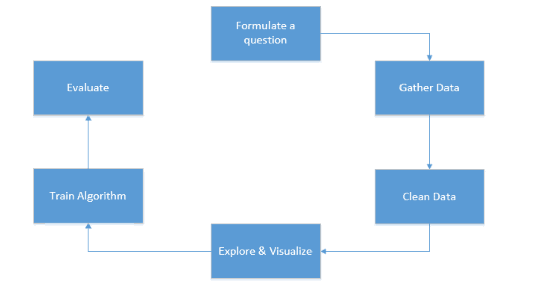
To create a successful machine learning model, you need to follow some steps:

  • Formulate the question
  • Gather and clean the data
  • Visualise the data
  • Train the algorithm
  • Evaluate the result based on the requirements.

To solve the problem, you are going to follow these steps:

Formulate a question

The question is the same example you saw before given the movie budget and revenue. The question is “How much money/revenue is the movie going to make?”

Gather data

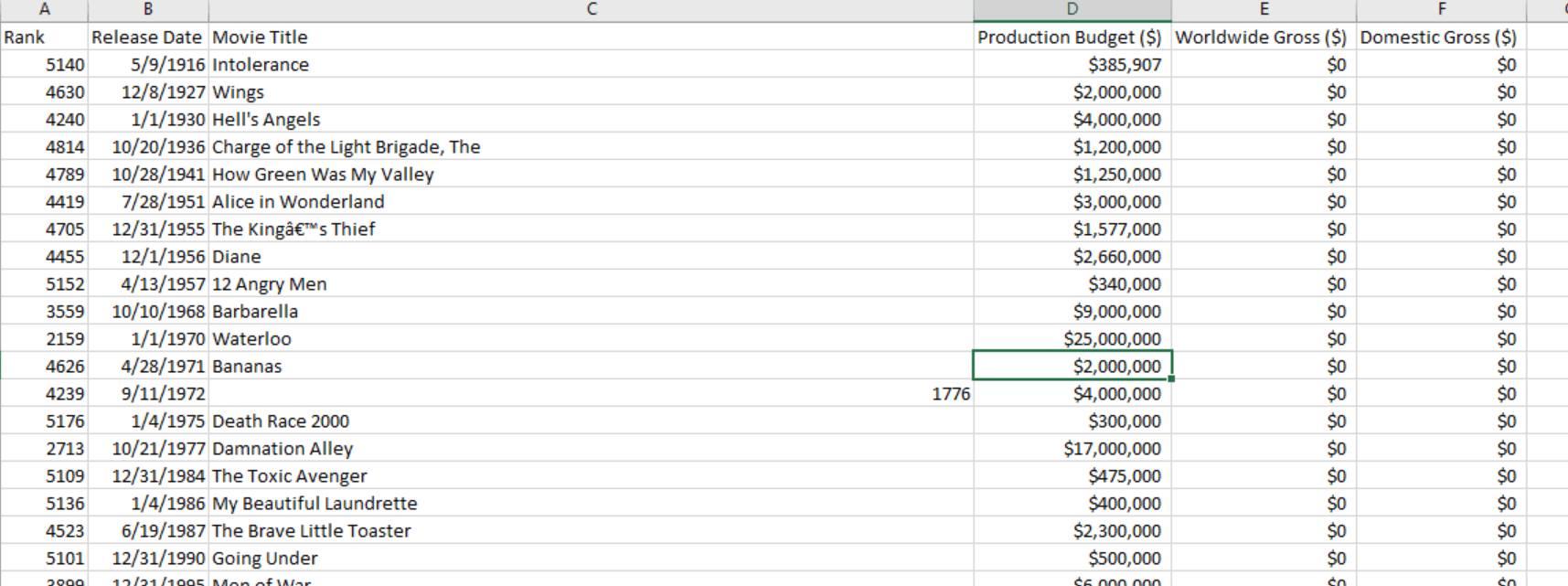
To perform the analysis on the data, you need the movie budget in USD and movie revenue in USD. You can use this website to gather the data. All you have to do is download the data and open it in Excel for your research. (To make it easier, you can download the data from here as well.)

Clean the data

The next step is cleaning the wrong data. You might have noticed that the data in the Excel sheet contains a $0 amount in some cases.

The reason for this might be because the movie dates are in the future or the movie never came out. There might be many more reasons to have a $0 amount there, so for now, delete these $0 rows so that they don’t cause any false failures in the analysis and focus on the ones which have concrete results.

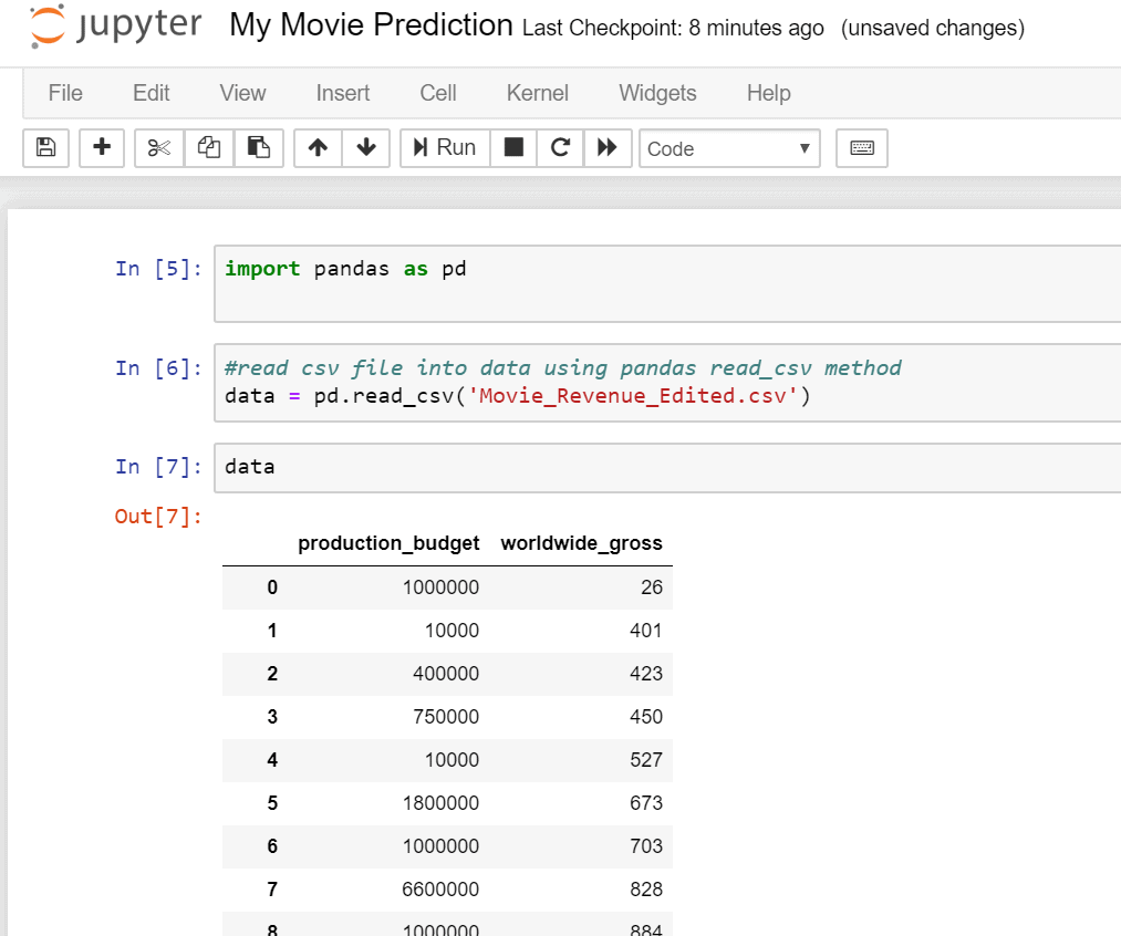
As discussed before, the focus will be just on the two columns production budget and worldwide gross because these are the columns that you will plot on the graph. After cleaning the data, removing the $ signs and renaming column names, this is how my Movie_Revenue_Edited looks:

Explore and Visualize

Now it’s time to visualise how the production budget and worldwide gross are related to each other. To do so, import the .csv file now so that you can do some magic on it. For this, click on the Jupyter logo, and it will take you to a screen. Click on Upload to upload the Movie_Revenue_Edited.csv file. 

The next step is to start with a fresh notebook. In the Jupyter notebook, go to the File Menu-> New Notebook -> Python 3. This will open a new instance of Python notebook for you. I have renamed my notebook to My Movie Prediction. (You can also download the completed Movie Linear Regression Notebook.)

Now to access the csv file into the notebook, you need to use the Pandas module. Pandas is a prebuilt data science library that lets you do fast data analysis as well as data cleaning. It is built on the top of a famous data science library called NumPy. Pandas work with wide variety of data sources such as Excel, CSV, SQL file. In each cell, you can write either markup or code. You can select a cell with code and run it to get the results right in the notebook.

Here’s an example of importing the file and displaying the data (be sure to enter the code into the individual cells as shown in the image):

import pandas as pd
#read csv file into data using pandas read_csv method
data = pd.read_csv('Movie_Revenue_Edited.csv')
data

The next step is to load the data into the X and Y axis for the plot. X is going to be production_budget and Y will contain the worldwide_gross from the datasheet. To serve this purpose, you will have to map the csv data into rows and columns. This can be achieved using Pandas Data Frame. Data Frames is a two-dimensional and heterogeneous tabular data structure with labelled axes, i.e., rows and columns. The data frames package must be imported before using them in the code, which is very similar to the way you import packages in JAVA and C#. Go back to the cell where you imported the Pandas library and add the new from line. After adding the code, rerun the cell.

import pandas as pd
from pandas import DataFrame as df


Now to get the data loaded into the X and Y axes, you will load the data frame with production_budget and Y-axis with worldwide_gross. Make sure you provide the same column name as that of your input csv data. The code will look something like this:

X = df(data, columns=['production_budget'])
Y = df(data, columns=['worldwide_gross'])

Now that you have successfully separated the data, you can visualise it. For this, you will need to import another module called Matplotlib. It has a rich library of graphing and plotting functionality. You will use the pyplot feature from this module. Just add the import statement to import the correct module. Make sure that you hit the Run button whenever you write new code to execute the cell’s code.

import pandas as pd
from pandas import DataFrame as df
import matplotlib.pyplot as mp


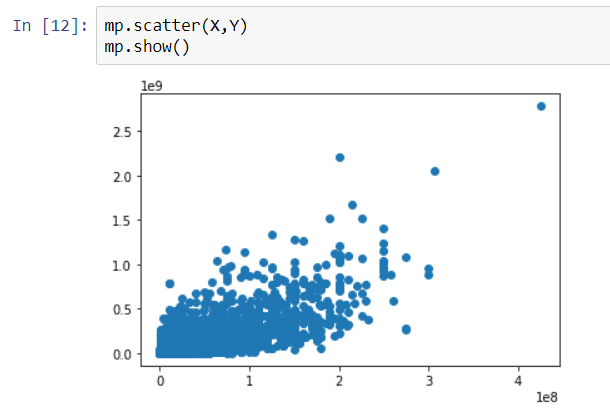
In a new cell, you will write code to print the plot. You will use Scatter Plots here as they help you find the correlation between these two variables. To display the plot, you will use the pyplot.show() method.

mp.scatter(X,Y)
mp.show()


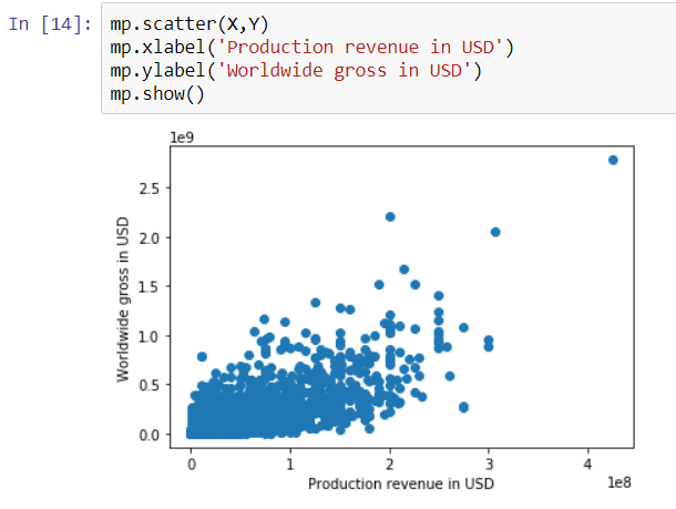
To make the chart more readable, annotate the X and Y axes. This can be done using pyplot’s xlabel and ylabel methods.

mp.scatter(X,Y)
mp.xlabel('Production revenue in USD')
mp.ylabel('Worldwide gross in USD')
mp.show()


Train the algorithm

Now you can run the regression on the plot to analyse the results. The main goal here is to achieve a straight line or the line of predicted values that would act as a reference to analyse any future predictions. As you might have realised by now, there are several modules that provide different functionality. To run the regression, you will use Scikit-learn which is a very popular machine learning module. Back in the import cell, add the new line to import linear regression from the Scikit-learn module and rerun.

import pandas as pd 
from pandas import DataFrame as df 
import matplotlib.pyplot as mp
from sklearn.linear_model import LinearRegression


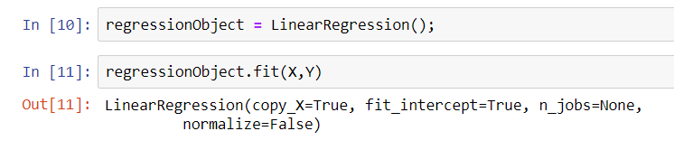
Scikit-learn helps you create a linear regression model. Since the task of running the linear regression is done by an object, you will need to create a new object, in this case with the name regressionObject. The Fit method can be used to fit the regression model to the data. In other words, you have to make the model learn using the training data. For this purpose, use the fit method as shown below.

regressionObject = LinearRegression();
regressionObject.fit(X,Y)


Once your model is trained with the training dataset, you can predict the value for Y using the regression object. The predict method will help you predict values for Y for each X.

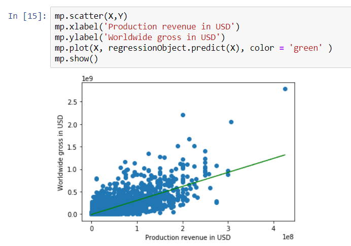
So yPredicted will be equal to regressionObject.predict(X), and then yPredicted is used to build the regression line onto the plot using this statement. You will notice that I have used the green colour for the regression line, which shows up in the plot successfully. Change the previous cell so that it includes the plot.

mp.scatter(X,Y) 
mp.xlabel('Production revenue in USD') 
mp.ylabel('Worldwide gross in USD') 
mp.plot(X, regressionObject.predict(X), color = 'green')
mp.show


Analyse

As you can see from the plot, there is a positive relationship between the two values. As production revenue increases, there is an increase in worldwide gross. This means the rate of change of variable Y is proportional to the change in X. When the regression line is linear the equation of line is Y = aX + b, the a is the regression coefficient/slope of the line which signifies the variance of Y with change in values of X.

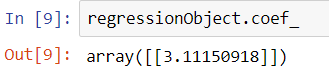
The positive regression coefficient (a) will tell you that there is a positive relationship between X and Y. The coefficient value can be determined using coef_ property on the regression object. For this map, the regression coefficient is 3.11, which means that for each USD spent for the movie production, you should get $3.11 in return.

regressionObject.coef_


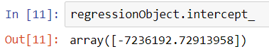
The next step is to calculate b the intercept_ of the line. This can be done by using intercept_ property on the regression object.

regressionObject.intercept_


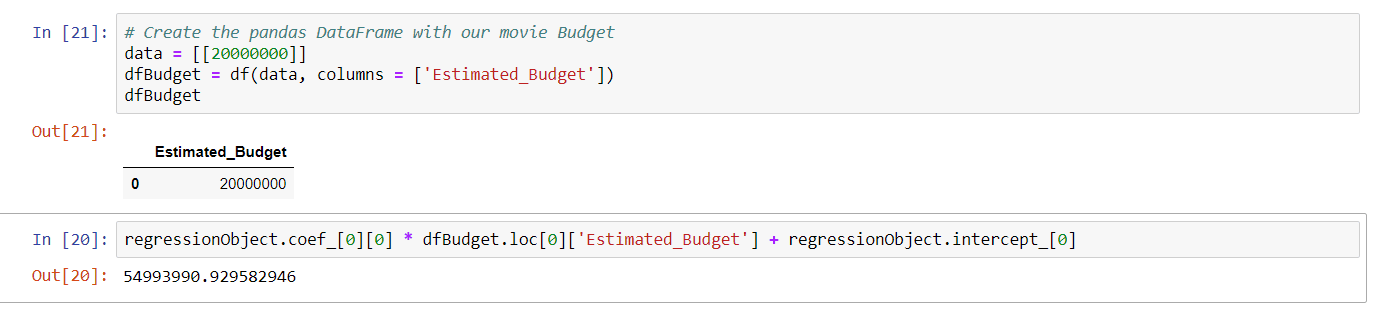
The generalized formula for a line is Y = aX + b. Now consider a hypothetical scenario where you want to predict the worldwide revenue that a movie made for $20 Million in production budget. The estimation can be found by substituting the values in the equation.

Y = 3.11150918 * 20,000,000 + (-7236192.72913958)
Y = 54,993,990.87086042

The above calculation can be done using the Python notebook as below:


# Create the pandas DataFrame with our movie Budget
data = [[20000000]]
dfBudget = df(data, columns = ['Estimated_Budget'])
dfBudget

regressionObject.coef_[0][0] * dfBudget.loc[0]['Estimated_Budget'] + regressionObject.intercept_[0]


The important thing to note here is the model is a hypothetical analysis of the data provided. The predictions are not 100% accurate, but there is a high possibility that the predictions would turn out to be true. Keep in mind that the model is a dramatic simplification of the real world.

Summary

This article provided an introduction to the concepts of machine learning, data science and linear regression. It demonstrated how to build and analyse the Machine Learning Linear Regression Model through various steps which will eventually enabled you to predict the outcome for practical problems.

References

https://hackernoon.com/the-ai-hierarchy-of-needs-18f111fcc007

https://towardsdatascience.com/linear-regression-detailed-view-ea73175f6e86

https://www.the-numbers.com/

http://www.data-analysis-in-python.org/


The post Building Machine Learning Models to Solve Practical Problems appeared first on Simple Talk.


from Simple Talk https://ift.tt/2lphBGg
via

Tuesday, September 24, 2019

SQL Server Management Studio is as Relevant as Ever

After fifteen years of heavy usage by developers and DBAs, it might seem like Microsoft’s free tool, SQL Server Management Studio, is about to go out of style. SSMS is no longer the cool new kid on the block: Microsoft has shown consistent effort to develop their new tool, Azure Data Studio (formerly known as SQL Operations Studio), since November 2017.  

It might seem like DBAs and devs should primarily learn Azure Data Studio, not SSMS, and that vendors should focus on developing new tooling only for Azure Data Studio. But when you look into the details, SSMS is as relevant as ever. 

Azure Data Studio shines where it specialises in unique functionality 

While both Azure Data Studio and SSMS each provide an interface to author queries and to execute them against relational database instances, I find that the user experience in Azure Data Studio is often not nearly as smooth as it is in SSMS. 

Where Azure Data Studio shows its value is in unique experiences: 

  • SQL Notebooks (based on Jupyter notebooks) which offer an experience of “interactive documentation” and more 
  • The ability for users to connect, manage, and query different database platforms, using tools like the PostgreSQL extension 
  • The ability for macOS or Linux users to run Azure Data Studio natively, without installing a Windows client 
  • The ability to work in other languages, such as PowerShell 

Azure Data Studio sometimes connects to SSMS 

One new Azure Data Studio feature I noticed in June 2019 is a Microsoft extension that allows the user to right-click on objects like databases and tables and view the Properties Dialog for the object. This dialogue is a Windows-only extension because behind the scenes Azure Data Studio is using parts of SSMS! This type of dependency is a strong signal that SSMS isn’t going away. 

SSMS is still under active development 

A major update to SQL Server Management Studio, SSMS 18.0, released in April 2019. This release included many improvements and new features. New features have been regularly added in the versions since this release as well. 

This pattern shows evidence to support Dinakar Nethi’s suggestion in his SSMS 18.0 release announcement that we should “think of these two tools not as separate tools doing different things, but as one integrated tool. Each tool has different experiences built into it and can be launched from the other seamlessly.” 

Users love SSMS – vendors do, too 

SSMS provides a very rich experience and covers a vast number of features – and it’s free! It’s well established and incredibly popular with developers and DBAs. 

For this reason, vendors will continue to build new features for SSMS. 

For example, at Redgate, we’ve just released a major new extension for SQL Change Automation in SSMS, which allows users to author changes in a migrations-first approach to development. We wish to empower teams to collaborate both across Visual Studio and other IDEs, and we recognise that SSMS continues to be the primary tool for Microsoft Data Platform DBAs and many developers. 

Where do we go from here? 

SSMS remains the primary tool for SQL Server specialists. Azure Data Studio is a terrific, complementary tool, with strong use cases for cross-platform experiences and SQL Notebooks. For new database administrators working with SQL Server, it continues to make sense to learn SSMS first. For more established users, we can enjoy working with both tools and enjoy the new features in Azure Data Studio without fear that our old friend SSMS is going away. 


Commentary Competition

Enjoyed the topic? Have a relevant anecdote? Disagree with the author? Leave your two cents on this post in the comments below, and our favourite response will win a $50 Amazon gift card. The competition closes two weeks from the date of publication, and the winner will be announced in the next Simple Talk newsletter.

The post SQL Server Management Studio is as Relevant as Ever appeared first on Simple Talk.


from Simple Talk https://ift.tt/2lcafGl
via

Tuesday, September 17, 2019

How to Use Parameters in PowerShell

Recently I had a client ask me to update a script in both production and UAT. He wanted any emails sent out to include the name of the environment. It was a simple request, and I supplied a simple solution. I just created a new variable:

$envname = "UAT"

After updating the script for the production environment, I then modified the subject line for any outgoing emails to include the new variable.

At the time though, I wanted to do this in a better way, and not just for this variable, but also for the others I use in the script. When I wrote this script, it was early in my days of writing PowerShell, so I simply hardcoded variables into it. It soon became apparent that this was less than optimal when I needed to move a script from Dev\UAT into production because certain variables would need to be updated between the environments.

Fortunately, like most languages, PowerShell permits the use of parameters, but, like many things in PowerShell, there’s more than one way of doing it. I will show you how to do it in two different ways and discuss why I prefer one method over the other.

Let’s Have an Argument

The first and arguably (see what I did there) the easiest way to get command line arguments is to write something like the following:

$param1=$args[0]
write-host $param1

If you run this from within the PowerShell ISE by pressing F5, nothing interesting will happen. This is a case where you will need to run the saved file from the ISE Console and supply a value for the argument.

To make sure PowerShell executes what you want, navigate in the command line to the same directory where you will save your scripts. Name the script Unnamed_Arguments_Example_1.ps1 and run it with the argument FOO. It will echo back FOO(The scripts for this article can be found here.)

.\Unnamed_Arguments_Example_1.ps1 FOO

You’ve probably already guessed that since $args is an array, you can access multiple values from the command line.

Save the following script as Unnamed_Arguments_Example_2.ps1. 

$servername=$args[0]
$envname=$args[1]
write-host "If this script were really going to do something, it would do it on $servername in the $envname environment"

Run it as follows:

.\Unnamed_Arguments_Example_2.ps1 HAL Odyssey

You should see:

One nice ability of reading the arguments this way is that you can pass in an arbitrary number of arguments if you need to. Save the following example as Unnamed_Arguments_Example_3.ps1

write-host "There are a total of $($args.count) arguments"
for ( $i = 0; $i -lt $args.count; $i++ ) {
    write-host "Argument  $i is $($args[$i])"
}

If you call it as follows:

.\Unnamed_Arguments_Example_3.ps1 foo bar baz

You should get:

The method works, but I would argue that it’s not ideal. For one thing, you can accidentally pass in parameters in the wrong order. For another, it doesn’t provide the user with any useful feedback. I will outline the preferred method below.

Using Named Parameters

Copy the following script and save it as Named_Parameters_Example_1.ps1.

param ($param1)
write-host $param1

Then run it.

.\Named_Parameters_Example_1.ps1

When you run it like this, nothing will happen.

But now enter:

.\Named_Parameters_Example_1.ps1 test

And you will see your script echo back the word test.

This is what you might expect, but say you had multiple parameters and wanted to make sure you had assigned the right value to each one. You might have trouble remembering their names and perhaps their order. But that’s OK; PowerShell is smart. Type in the same command as above but add a dash (-) at the end.

.\Named_Parameters_Example_1.ps1 -

PowerShell should now pop up a little dropdown that shows you the available parameters. In this case, you only have the one parameter, param1. Hit tab to autocomplete and enter the word test or any other word you want, and you should see something similar to:

.\Named_Parameters_Example_1.ps1 -param1 test

Now if you hit enter, you will again see the word test echoed.

If you run the script from directly inside PowerShell itself, as opposed to the ISE, tab completion will still show you the available parameters, but will not pop them up in a nice little display.

Create and save the following script as Named_Parameters_Example_2.ps1.

param ($servername, $envname)
write-host "If this script were really going to do something, it would do it on $servername in the $envname environment"

Note now you have two parameters.

By default, PowerShell will use the position of the parameters in the file to determine what the parameter is when you enter it. This means the following will work:

.\Named_Parameters_Example_2.ps1 HAL Odyssey

The result will be:

Here’s where the beauty of named parameters shines. Besides not having to remember what parameters the script may need, you don’t have to worry about the order in which they’re entered.

.\Named_Parameters_Example_2.ps1 -envname Odyssey -servername HAL

This will result in the exact same output as above, which is what you should expect:

If you used tab completion to enter the parameter names, what you will notice is once you’ve entered a value for one of the parameters (such as –envname above), when you try to use tab completion for another parameter, only the remaining parameters appear. In other words, PowerShell won’t let you enter the same parameter twice if you use tab completion.

If you do force the same parameter name twice, PowerShell will give you an error similar to:

One question that probably comes to mind at this point is how you would handle a parameter with a space in it. For example, how would you enter a file path like C:\path to file\File.ext.

The answer is simple; you can wrap the parameter in quotes:

.\Named_Parameters_Example_2.ps1 -servername HAL -envname 'USS Odyssey'

The code will result in:

With the flexibility of PowerShell and quoting, you can do something like:

.\Named_Parameters_Example_2.ps1 -servername HAL -envname "'USS Odyssey'"

You’ll see this message back:

If you experiment with entering different values into the scripts above, you’ll notice that it doesn’t care if you type in a string or a number or pretty much anything you want. This may be a problem if you need to control the type of data the user is entering.

This leads to typing of your parameter variables. I generally do not do this for variables within PowerShell scripts themselves (because in most cases I’m controlling how those variables are being used), but I almost always ensure typing of my parameter variables so I can have some validation over my input.

Consider why this may be important. Save the following script as Named_Parameters_Example_3.ps1

param ([int] $anInt, $maybeanInt)
write-host "Adding $anint to itself results in: $($anInt + $anInt)"
write-host "But trying to add $maybeanInt to itself results in: $($maybeanInt + $maybeanInt)"

Now run it as follows:

.\Named_Parameters_Example_3.ps1 -anInt 5 -maybeanInt 6

You will get the results you expect:

What if you don’t control the data being passed, and the passing program passes items in quoted strings?

To simulate that run the script with a slight modification:

.\Named_Parameters_Example_3.ps1 -anInt "5" -maybeanInt "6"

This will result in:

If you instead declare $maybeanInt as an [int] like you did $anInt, you can assure the two get added together, not concatenated.

However, keep in mind if someone tries to call the same script with an actual string such as:

.\Named_Parameters_Example_3.ps1 Foo 6

It will return a gross error message, so this can be a double-edged sword.

Using Defaults

When running a script, I prefer to make it require as little typing as possible and to eliminate errors where I can. This means that I try to use defaults.

Modify the Named_Parameters_Example_2.ps1 script as follows and save it as Named_Parameters_Example_4.ps1

param ($servername, $envname='Odyessy')
write-host "If this script were really going to do something, it would do it on $servername in the $envname environment"

And then run it as follows:

.\Named_Parameters_Example_4.ps1 -servername HAL

Do not bother to enter the environment name. You should get:

This isn’t much savings in typing but does make it a bit easier and does mean that you don’t have to remember how to spell Odyssey!

There may also be cases where you don’t want a default parameter, but you absolutely want to make sure a value is entered. You can do this by testing to see if the parameter is null and then prompting the user for input.

Save the following script as Named_Parameters_Example_5.ps1.

param ($servername, $envname='Odyessy')
if ($servername -eq $null) {
$servername = read-host -Prompt "Please enter a servername" 
}
write-host "If this script were really going to do something, it would do it on $servername in the $envname environment"

You will notice that this combines both, a default parameter and testing the see if the $servername is null and if it is, prompting the user to enter a value.

You can run this from the command line in multiple ways:

.\Named_Parameters_Example_5.ps1 -servername HAL

It will do exactly what you think: use the passed in servername value of HAL and the default environment of Odyssey.

But you could also run it as:

.\Named_Parameters_Example_5.ps1 -envname Discovery

And in this case, it will override the default parameter for the environment with Discovery, and it will prompt the user for the computer name. To me, this is the best of both worlds.

There is another way of ensuring your users enter a parameter when it’s mandatory.

Save the following as Named_Parameters_Example_6.ps1

param ([Parameter(Mandatory)]$servername, $envname='Odyessy')
write-host "If this script were really going to do something, it would do it on $servername in the $envname environment"

and run it as follows:

.\Named_Parameters_Example_6.ps1

You’ll notice it forces you to enter the servername because you made that mandatory, but it still used the default environment name of Odyssey.

You can still enter the parameter on the command line too:

.\Named_Parameters_Example_6.ps1  -servername HAL -envname Discovery

And PowerShell won’t prompt for the servername since it’s already there.

Using an Unknown Number of Arguments

Generally, I find using named parameters far superior over merely reading the arguments from the command line. One area that reading the arguments is a tad easier is when you need the ability to handle an unknown number of arguments.

For example, save the following script as Unnamed_Arguments_Example_4.ps1

write-host "There are a total of $($args.count) arguments"
for ( $i = 0; $i -lt $args.count; $i++ ) {
    $diskdata = get-PSdrive $args[$i] | Select-Object Used,Free
    write-host "$($args[$i]) has  $($diskdata.Used) Used and $($diskdata.Free) free"
}

Then call it as follows:

.\Unnamed_Arguments_Example_4.ps1 C D E

You will get back results for the amount of space free on the drive letters you list. As you can see, you can enter as many drive letters as you want.

One attempt to write this using named parameters might look like:

param($drive1, $drive2, $drive3)
$diskdata = get-PSdrive $drive1 | Select-Object Used,Free
write-host "$($drive1) has  $($diskdata.Used) Used and $($diskdata.Free) free"
if ($drive2 -ne $null) {
$diskdata = get-PSdrive $drive2 | Select-Object Used,Free
write-host "$($drive2) has  $($diskdata.Used) Used and $($diskdata.Free) free"
    if ($drive3 -ne $null) {
    $diskdata = get-PSdrive $drive3 | Select-Object Used,Free
    write-host "$($drive3) has  $($diskdata.Used) Used and $($diskdata.Free) free"
    }
    else
    { return}
}
else
{return} # don't bother testing for drive3 since we didn't even have drive 3

As you can see, that gets ugly fairly quickly as you would have to handle up to 26 drive letters.

Fortunately, there’s a better way to handle this using named parameters. Save the following as Named_Parameters_Example_7.ps1

param($drives)
foreach ($drive in $drives) 
{
    $diskdata = get-PSdrive $drive | Select-Object Used,Free
    write-host "$($drive) has  $($diskdata.Used) Used and $($diskdata.Free) free"
}

If you want to check the space on a single drive, then you call this as you would expect:

.\Named_Parameters_Example_7.ps1 C

On the other hand, if you want to test multiple drives, you can pass an array of strings.

This can be done one of two ways:

.\Named_Parameters_Example_7.ps1 C,D,E

Note that there are commas separating the drive letters, not spaces. This lets PowerShell know that this is all one parameter. (An interesting side note: if you do put a space after comma, it will still treat the list of drive letters as a single parameter, the comma basically eats the space.)

If you want to be a bit more explicit in what you’re doing, you can also pass the values in as an array:

.\Named_Parameters_Example_7.ps1 @("C","D","E")

Note that in this case, you do have to qualify the drive letters as strings by using quotes around them.

Conclusion

Hopefully, this article has given you some insight into the two methods of passing in variables to PowerShell scripts. This ability, combined with the ability to read JSON files in a previous article should give you a great deal of power to be able to control what your scripts do and how they operate. And now I have a script to rewrite!


The post How to Use Parameters in PowerShell appeared first on Simple Talk.


from Simple Talk https://ift.tt/31tICbD
via

Wednesday, September 11, 2019

The Data-Philes Team Meet the Time Traveler

The year is 1999, somewhere in Cambridge, UK. Kathi, a member of the Data-Philes team, is reading a memo sent from her manager. The memo talks about someone who disrupted a project management meeting in London. He claims he is from 20 years in the future. Chris walks in.

Chris: Kathi, have you seen the latest assignment from Simon? If we leave now,  we can be at the facility where the time traveler is being held in a few minutes. Maybe he can share some of the news about 2019, like where to buy the best flying car.

Kathi: A few minutes! Do you have a transporter that I don’t know about? Chris, obviously, this man is suffering from delusions. There is no reason interview him. Instead, I just heard that SQL Server 7 was released, and I would like to spend some time checking it out.

Chris: Ya know, Kathi, you don’t even need a DBA when you use SQL Server 7.

Kathi: Ugh. I need to start brushing up on Oracle. All the SQL 6.5s will probably be upgraded within a year, and I won’t have a job!

Chris: There is something really odd about our time traveler. You wouldn’t believe some of the things he said at that meeting!

Kathi: Like what?

Chris: Well, first, he said that the way the company builds software is all wrong.

Kathi: Aren’t they using Waterfall methodology?

Chris: That’s just it. They are using it.

Kathi: So, why is that wrong?

Chris: He says that in the future, companies will embrace something called DevOps. Instead of building the entire project and releasing it all at once, they will deploy code daily, maybe even several times a day! Developers and operations teams, including DBAs, will work together to make sure that deployments run smoothly.

Kathi: DevOps? That sounds like science fiction! Obviously, this man has watched a few too many Star Trek episodes!

Chris: It gets better. He started talking about cloning databases to save space and time for developers.

Kathi: See, there you go. Why would anyone care about saving space and time? The biggest database I’ve worked with was just a few gigabytes. Yes, it’s a pain to copy for developers and setting everything up takes a few days, but we only have to do it a couple of times a year. We are careful to keep the database stable and not let too many changes sneak in.

Chris: That’s what’s so amazing. He said that, in 20 years, it will not be unusual to have terabyte databases! With cloning, even a terabyte database can be delivered to a developer in seconds! And, it doesn’t take up much room on the dev’s hard drive.

Kathi: Like I said: too much Star Trek! And, of course, when we need to set up a brand-new environment, it only takes a few months to order the hardware, build it, and get everything installed. It’s not a big deal as long as there is space for the new server in the basement server room.

Chris: Virtualization will be popular, too, so you won’t have to order hardware for every project.

Kathi: Well, SQL Server will never run on a virtual machine!

Chris: He also mentioned that the company should do everything they can to prevent data breaches, especially since so much data will live in the cloud.

Kathi: What is a data breach? Data in the cloud? Now I know this guy is delusional. That sounds like something from a Star Wars movie or maybe The Matrix.

Chris: Evidently, in the future, it is not unusual for the data from a major company to be stolen. Names, addresses, credit card numbers, all that in the hands of thieves! If only they would use their powers for good and not evil!

Kathi: Is there any way to protect this type of sensitive information in the future?

Chris: Yes, he mentions that companies can use data masking software to sanitize personal information before giving the databases to developers.

Kathi: That’s amazing, but it sounds like so much work.

Chris: This is why I think this guy might be telling the truth. He mentioned that there are tools in the future that make automating this easier than it sounds. He even managed to bring back some of these tools to demonstrate to the team.

Kathi: Now, that I’d like to see…

The post The Data-Philes Team Meet the Time Traveler appeared first on Simple Talk.


from Simple Talk https://ift.tt/32Abajz
via

SQL Server 2019 Graph Database and SHORTEST_PATH

My crystal ball seems to be working again: The new addition to SQL Server 2019, shortest_path, was the subject of many of the technical sessions I delivered as one of the missing features of SQL Server Graph Database.

I will use an example that is similar to the first article I wrote on this topic. You can create the database and tables needed for this article using this script. Maybe you would also like to read the previous blog post about some recent improvements in Graph Databases.

Since the data is essentially a graph, a solution to visually show the results is helpful. An application like Gephi to can be used to view the graph. (You can download this application here.) To use Gephi with SQL Server, make sure that the TCP/IP protocol and mixed authentication are enabled. The app only supports SQL authentication, so you will need a SQL Server login to connect.

Using Gephi

Follow these steps to view the graph in Gephi.

  • After opening Gephi, select New Project on the Welcome screen
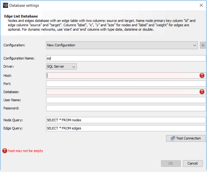
  • On the File menu, select Import Database->Edge List. This will open the Database settings screen.

A screenshot of a cell phone Description automatically generated

  • In the Configuration Name field, create a name for the configuration, such as SQLServer2019.
  • In the Driver field, select SQL Server.
  • In the Host field, insert the machine/instance name of your SQL Server
  • In the Port field, enter the port used, typically 1433. If you’re not sure, look for the port number in the SQL Server Configuration Manager program.
  • In the Database field, insert the name of the database which contains the graph tables which is probably GraphDemo if you have been following along
  • In the Username field, enter the username of a SQL Server login with SELECT permission to the tables in the GraphDemo database.
  • In the Password field, insert the password for the SQL login.

In addition to the configuration required to connect to SQL Server, the Database settings screen also requires two queries: One to retrieve the list of nodes from the server and another to retrieve the list of edges from the server. I’ll explain those queries next.

The screen itself contains information at the top of the dialog about the columns the queries need to return, and it’s important to notice these columns are case sensitive.

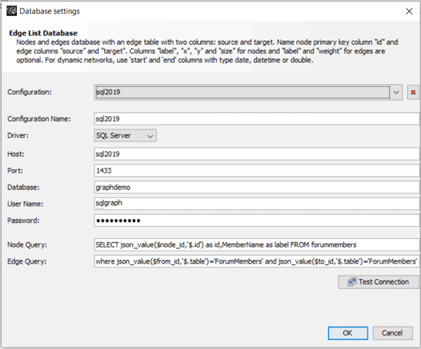
The nodes table in SQL Server has the pseudo-column $node_id, which is a JSON column. A good option is to extract the id from the JSON and use the MemberName as the label for the node. The query will look like this:

SELECT Json_value($node_id, '$.id') AS id, 
       membername                   AS label 
FROM   forummembers 

The edge query has also to extract the id from  $to_node and $from_node, but besides that, you need to filter the nodes returned, because the nodes table from the previous article has a relation between two members and between members and messages. For this example, return only the relation between two members. Here is the query:

SELECT Json_value($from_id, '$.id') AS source, 
       Json_value($to_id, '$.id')   AS target 
FROM   likes 
WHERE Json_value($from_id, '$.table') = 'ForumMembers' 
      AND Json_value($to_id, '$.table') = 'ForumMembers' 

It’s important to note that the source and target id’s in the edge query need to match with the ids in the node query. There are some additional columns that could be used, but for this example, you’ll only need these.

The final configuration will look similar to the following image:

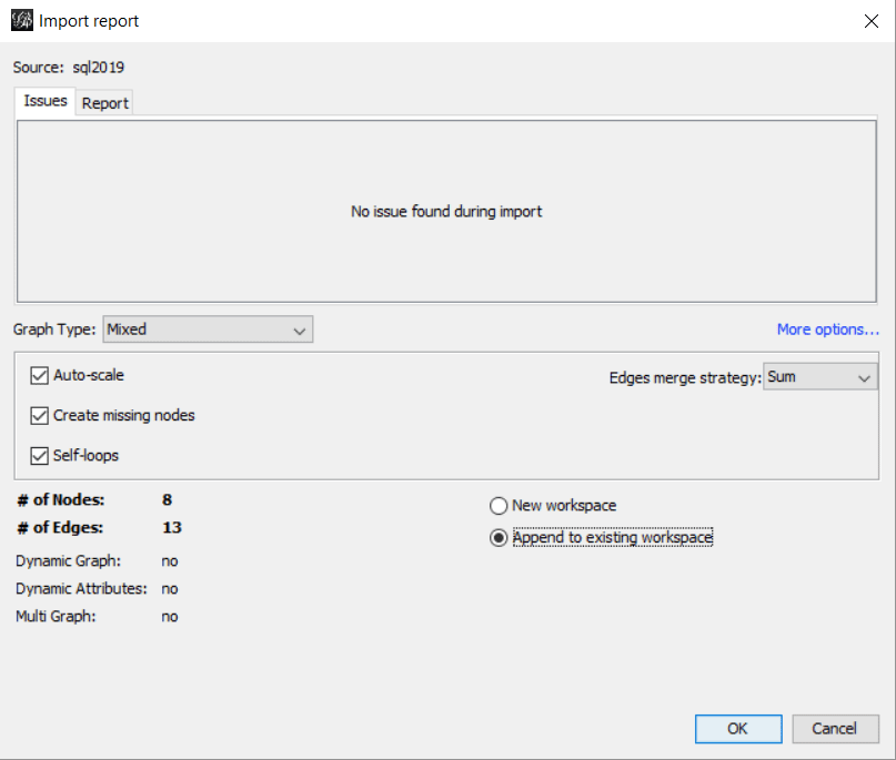
After you click OK, the next window, Import Report, involves many details but they will not be covered in this article. What’s important here is the number of nodes and edges found, confirming that the queries are correct. However, there is only a single step to be done on this screen:

Select the option Append to existing workspace.

A screenshot of a cell phone Description automatically generated

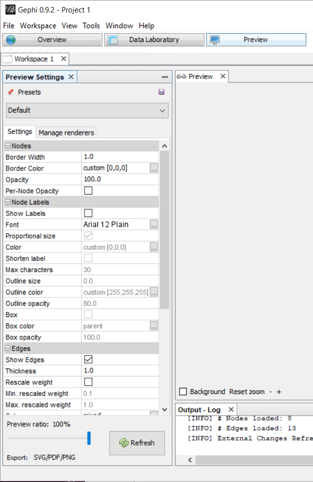
After this first screen, you will see the Workspace1 and Preview tabs and Preview Settings window. It’s time to build the graph.

A screenshot of a social media post Description automatically generated

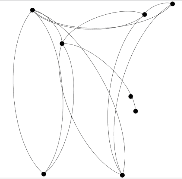
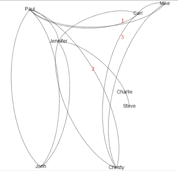
Click on the Refresh button inside the Preview Settings pane. This will result in an image similar to the one below. Note that yours may look different, but in the next step, you can verify that the nodes are connected correctly.

A picture containing sky, kite, water, outdoor Description automatically generated

Improve this graph just a bit by making these changes in the Preview Settings tab.

  • Change the Opacity property to 0 under Nodes.
  • Mark the Show Labels property under Node Labels.
  • Change the Outline opacity under Node Labels to 0

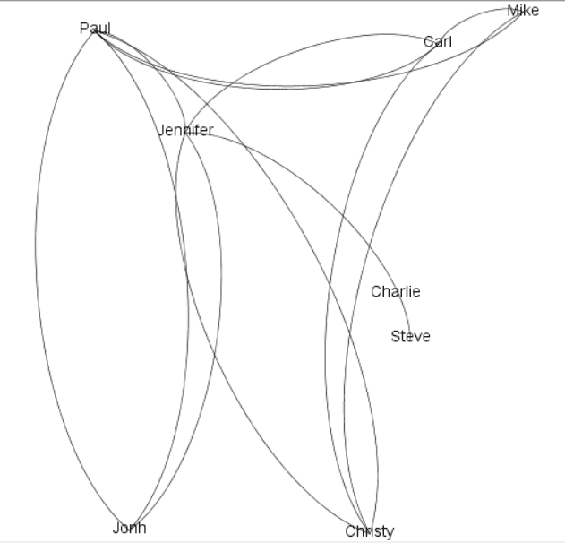
After clicking refresh, the graph will change to something like the image below:

A close up of a map Description automatically generated

As you may notice, even a simple graph with a small amount of data can be quite complex to identify information such as the shortest path between two nodes in the graph. That’s why you need a tool to calculate this, and SQL Server 2019 can make this kind of calculation.

Calculating the Path

When you think about a function to calculate the shortest path between two points, you may think that it will be a simple function. To make this calculation work, however, you need way more than a simple function. You must establish paths among the graph data. The data has many paths, and each one has many nodes with a beginning and an end. Each path is a group of nodes, in some ways like the group by function.

One similarity, for example, is that you can’t read the column directly from the path. You need to apply aggregation functions to the set of nodes that are part of the path to read the information.

The syntax to build this query resembles the GROUP BY clause, requiring you to use aggregate functions to make calculations on every (shortest) path of nodes, getting grouped results.

To make this simpler, start to build the query over the model piece by piece. First, the From clause

FROM 
    ForumMembers P1, 
    ForumMembers FOR PATH as P2, 
    Likes FOR PATH as IPO

The FOR PATH expression in the edge and node tables indicates these tables will be used to calculate paths, a grouping, in other words. Over the columns of these particular tables you can only apply aggregation functions; you can’t retrieve the columns directly.

You may have noticed the node table appears twice in the query, one using the FOR PATH and another without using the FOR PATH. Since you can’t retrieve columns directly from the FOR PATH tables, you can include the nodes table twice to retrieve individual values of the node columns, usually for the start node of the path.

Now analyse the list of columns and expressions in the SELECT list:

SELECT 
    P1.MemberID, 
    P1.MemberName, 
    STRING_AGG(P2.MemberName,
        '->') WITHIN GROUP (GRAPH PATH) AS [MemberName], 
    LAST_VALUE(P2.MemberName) WITHIN GROUP (GRAPH PATH) 
        AS FinalMemberName, 
    COUNT(P2.MemberId) WITHIN GROUP (GRAPH PATH) AS Levels

The first two columns come from the P1 table, which is not marked as FOR PATH. The MemberID and MemberName columns are from the first node of the path. The WHERE clause will also expose this.

The other three expressions use aggregate functions. They use the following functions:

Count: is a well know aggregate function

STRING_AGG: was introduced in a recent version of SQL Server and can be used to concatenate string values

LAST_VALUE: is a windowing function, but it can be used with any kind of aggregation, including a graph path.

Besides each aggregation function, you have the WITHIN GROUP (GRAPH PATH) statement, a special statement created for the grouping generated by the shortest_path function.

Finally, here’s the WHERE clause:

WHERE MATCH(SHORTEST_PATH(P1(-(IPO)->P2)+))

It’s like a regular MATCH clause that you already know about, but using the new function, SHORTEST_PATH. The first table, which is not part of the grouping, is related to the edge and node tables, which is part of the grouping. The edge and second node tables appear between parenthesis. The SHORTEST_PATH function understands this as an instruction to use recursion, creating the groups.

The ‘+‘ symbol indicates that you would like information about the entire path between each member of P1 and P2, without limiting the number of hops

Here’s the final query:

SELECT 
    P1.MemberID, 
    P1.MemberName, 
    STRING_AGG(P2.MemberName,
       '->') WITHIN GROUP (GRAPH PATH) AS [MemberName], 
    LAST_VALUE(P2.MemberName) WITHIN GROUP (GRAPH PATH) 
       AS FinalMemberName, 
    COUNT(P2.MemberId) WITHIN GROUP (GRAPH PATH) AS Levels 
  FROM 
    ForumMembers P1, 
    ForumMembers FOR PATH as P2, 
    Likes FOR PATH as IPO 
  WHERE MATCH(SHORTEST_PATH(P1(-(IPO)->P2)+));

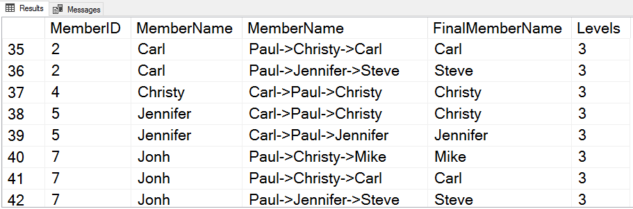
The image below gives an idea of the result. You have the information about the first member of the path, you have the entire path (not including the first member) created by the function STRING_AGG, you have the last name of the path created by the LAST_VALUE function, and you also have the number of levels in the path, created by the function COUNT

You may be wondering about how Carl connects to Carl. This image shows the path:

Performance

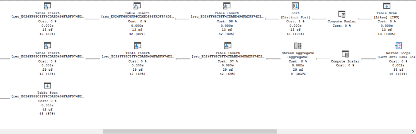
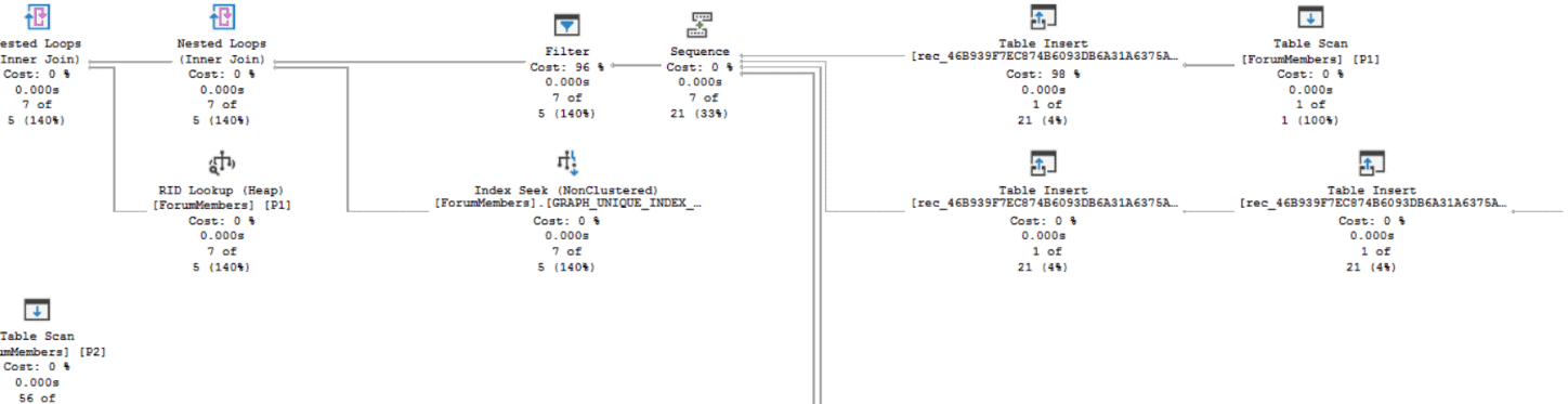
The execution plan is big. There is no doubt that you will need to take care when using it in large environments. The full execution plan doesn’t fit here, but you may notice by the piece below that the plan makes extensive use of tempdb.

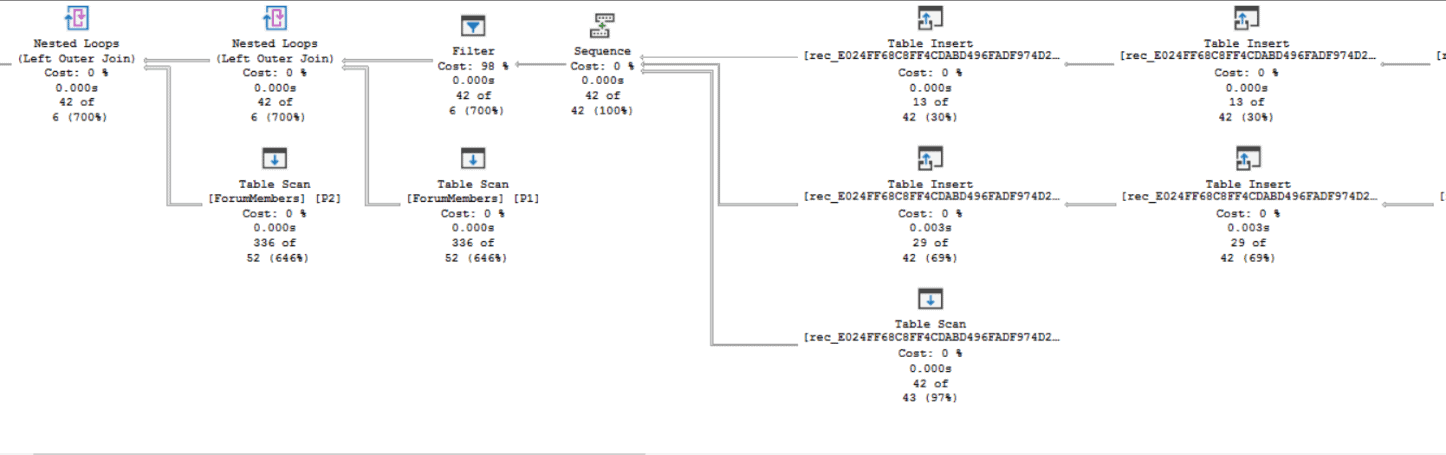
You may notice the following details in the execution plan:

  • It starts with the edge table
  • It creates three temporary tables from the edge table. You will see many table operations in the plan, but checking the names, you will notice there are only three

A screenshot of a computer Description automatically generated

  • It joins one of the temporary tables with the edge table, the nodes table and a second temporary table, aggregating the result and inserting in the temporary tables
  • It has a Sequence operator, which then is joined with the node table to get the results

A screenshot of a computer Description automatically generated

Filtering

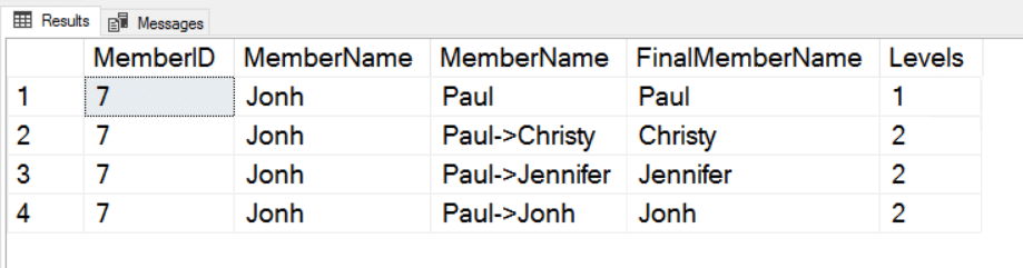
By adding one more predicate, you can view just the paths starting from one forum member:

SELECT 
   P1.MemberID, 
   P1.MemberName,
   STRING_AGG(P2.MemberName,'->') WITHIN GROUP 
       (GRAPH PATH) AS [MemberName],
   LAST_VALUE(P2.MemberName) WITHIN GROUP (GRAPH PATH) 
        AS FinalMemberName,
   COUNT(P2.MemberId) WITHIN GROUP (GRAPH PATH) AS Levels
FROM ForumMembers P1,
         ForumMembers FOR PATH as P2,
         Likes FOR PATH as IPO
WHERE MATCH(SHORTEST_PATH(P1(-(IPO)->P2)+))
          AND p1.MemberID=7;

A screenshot of a social media post Description automatically generated

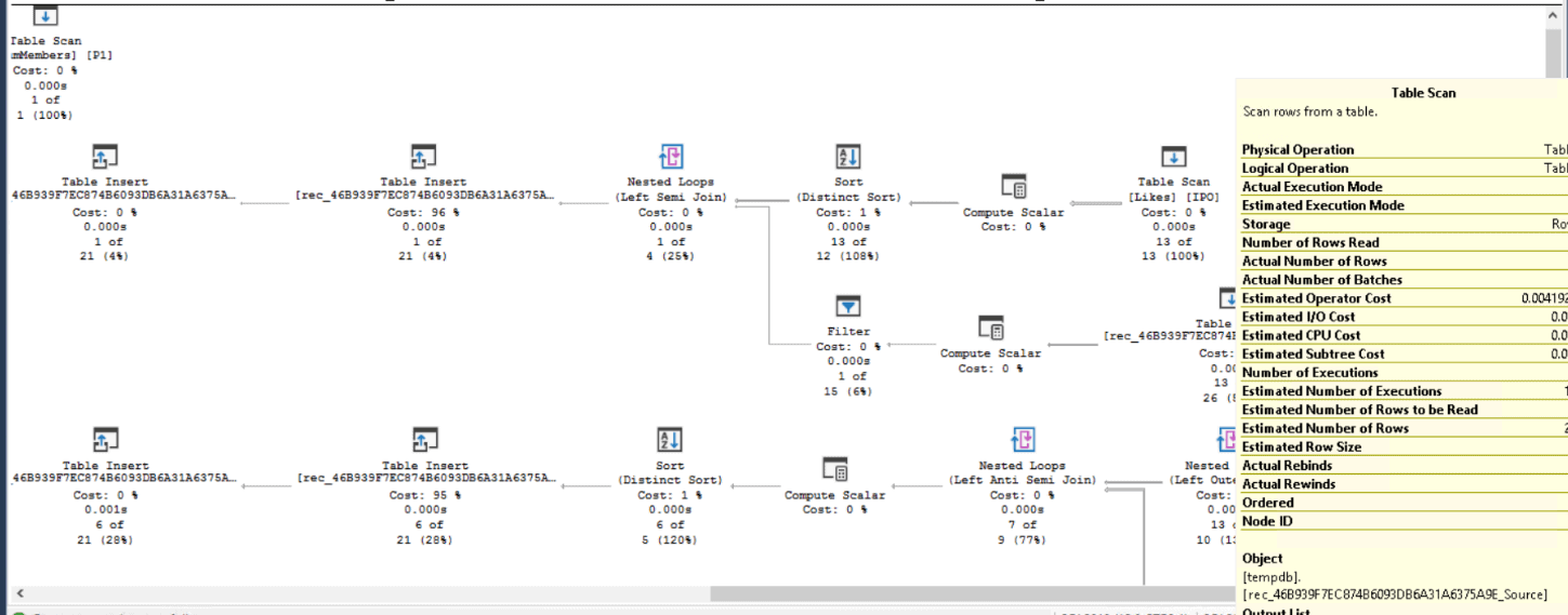
The execution plan changes. You may notice the following:

  • The sequence is still the middle of the execution plan
  • The plan starts by the node, not the edge
  • After the sequence, the Query Optimizer is able to use an index for one of the nodes

A screenshot of a video game Description automatically generated

  • There is a fourth temporary table, called Source
  • The number of paths before the sequence increases

A screenshot of a cell phone Description automatically generated

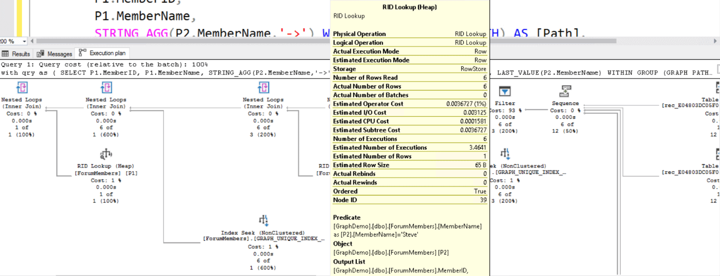
If you would like to see only the path between Jonh and Steve, you may be surprised that you have to separate the query into a CTE or subquery and filter the results. One reason is that a windowing function cannot be directly filtered. The MATCH statement doesn’t offer a solution either, you can’t filter by a P2 field, for example, because it’s marked as FOR PATH.

WITH qry AS (
  SELECT 
   P1.MemberID, 
   P1.MemberName,
   STRING_AGG(P2.MemberName,'->') WITHIN GROUP (GRAPH PATH) 
     AS [Path],
   LAST_VALUE(P2.MemberName) WITHIN GROUP (GRAPH PATH) 
     AS FinalMemberName,
   COUNT(P2.MemberId) WITHIN GROUP (GRAPH PATH) AS Levels
  FROM
   ForumMembers P1,
   ForumMembers FOR PATH as P2,
   Likes FOR PATH as IPO
  WHERE MATCH(SHORTEST_PATH(P1(-(IPO)->P2)+))
   and p1.MemberID=7)
SELECT * FROM qry 
WHERE FinalMemberName='Steve';

It’s not difficult to predict: The query plan is bad. You are calculating the path from Jonh to all other members and only after this does the filter kick in to get the path between Jonh and Steve. In the image below you may notice the filter for Steve only after the sequence, after calculating all the paths from Jonh

A screenshot of a cell phone Description automatically generated

You may have already noticed the + symbol in the Match clause. It means you allow an unlimited number of hops. However, you can use a slightly different syntax to find all the forum members that are, for example, up to two hops away from others:

SELECT 
   P1.MemberID, 
   P1.MemberName,
   STRING_AGG(P2.MemberName,'->') WITHIN GROUP (GRAPH PATH) 
      AS [MemberName],
   LAST_VALUE(P2.MemberName) WITHIN GROUP (GRAPH PATH) 
      AS FinalMemberName,
   COUNT(P2.MemberId) WITHIN GROUP (GRAPH PATH) AS Levels
FROM
   ForumMembers P1,
   ForumMembers FOR PATH as P2,
   Likes FOR PATH as IPO
WHERE MATCH(SHORTEST_PATH(P1(-(IPO)->P2){1,2}));

However, the start needs always to be 1. If you want to see the people that are an exact number of hops from other, once again you will need to filter the result of the query:

WITH qry as
(
  SELECT 
   P1.MemberID, 
   P1.MemberName,
   STRING_AGG(P2.MemberName,'->') WITHIN GROUP (GRAPH PATH) AS [path],
   LAST_VALUE(P2.MemberName) WITHIN GROUP (GRAPH PATH) AS FinalMemberName,
   COUNT(P2.MemberId) WITHIN GROUP (GRAPH PATH) AS Levels
  FROM
   ForumMembers P1,
   ForumMembers FOR PATH as P2,
   Likes FOR PATH as IPO
  WHERE MATCH(SHORTEST_PATH(P1(-(IPO)->P2){1,2}))
        )
SELECT * FROM qry WHERE levels=2;

The shortest_path function is a great new feature for the SQL Server graph database, but being unable to filter the end node or the exact number of hops without performing the entire calculation and only then filter the result is still a problem for query performance.

Indexing

You can create indexes on the pseudo-columns of the edge and nodes. Considering the execution plans you saw, you can create the following clustered index for the edge:

CREATE CLUSTERED INDEX indLikes ON likes($from_id,$to_id);

For the nodes, on the other hand, the index didn’t help so much. If you create a clustered index, it will result in a scan operation. If you create a non-clustered index, you would need to include all the columns involved in the operation. It may sound a bit strange, but one of the columns is the graph_id. There is no pseudo-column for the graph_id in the nodes table. There is one function to retrieve the graph_id, GRAPH_ID_FROM_NODE_ID, but you can’t use this function to create a computed column. This instruction bellow, for example, will fail:

ALTER TABLE forumMembers ADD graph_id 
AS (GRAPH_ID_FROM_NODE_ID($node_id))
PERSISTED;

On the other hand, for the queries where you are filtering for the start member, a non-clustered index on the member id helps:

CREATE NONCLUSTERED INDEX indMembers ON ForumMembers(memberid);

There is not much news about the more complex situations filtering by levels or end node: It’s an additional filter after all the calculations of shortest_path.

Conclusion

The function shortest_path is an excellent addition to the graph database features; however, the two limitations it has may create heavy queries in the environment:

  • You can’t specify an end node.
  • You can’t specify a start number of hops which would allow selecting an exact number of hops with same start and end.

The post SQL Server 2019 Graph Database and SHORTEST_PATH appeared first on Simple Talk.


from Simple Talk https://ift.tt/2Q3EbTC
via

Tuesday, September 10, 2019

Introduction to DevOps: Security, Privacy, and Compliance

The series so far:

  1. Introduction to DevOps: The Evolving World of Application Delivery
  2. Introduction to DevOps: The Application Delivery Pipeline
  3. Introduction to DevOps: DevOps and the Database
  4. Introduction to DevOps: Security, Privacy, and Compliance

A DevOps approach to application delivery offers a number of advantages over traditional methodologies, most notably faster and more efficient deployments, yet there’s nothing inherent in DevOps that promises more secure delivery or better protection for the applications and their data. In fact, DevOps can potentially lead to greater risks if security is not integrated into the development process right from the start. In today’s word of escalating cyberattacks and increased privacy regulations, security should be as much a part of application delivery as continuous testing and ongoing integration. Anything less could put your entire organization at risk.

DevOps Security Challenges

Cyberattacks are on the rise, and they’re becoming more sophisticated every day. If data is compromised, the consequences can have far-reaching implications, not only to the bottom line, but also to an organization’s long-term reputation.

Hackers know where to find security holes, how to exploit them, and what rewards they might be able to reap. They also recognize the opportunities that can result from accelerating software delivery without taking special care to protect applications and their data. Development teams that implement DevOps methodologies need to be particularly vigilant to guard against the many security challenges that come with delivering applications at a high velocity.

One of the biggest hurdles to security in a DevOps environment is the failure to factor in security right from the start—when planning and designing the application. Instead, security is treated as an afterthought, a clean-up operation, a reactive process separate from the primary development effort, resulting in slower application delivery or applications being released before they’ve been fully vetted.

Part of the reason for this disconnect is that traditional methods for ensuring application and data security do not fit easily within DevOps processes and, in fact, can inhibit operations. In addition, development and security teams often assume that, even with DevOps, it’s business as usual when it came to security, with the two teams operating independently of each other, often without coordinating efforts. The DevOps team will deliver the application, and the security team will identify and address any security issues, kicking the application back to the developers if it becomes necessary.

Unlike development and operations, where efforts merge together in a more organic fashion, development efforts can often seem at odds with the time-consuming processes that come with ensuring application security. On some DevOps teams, there can be a cultural resistance to security for fear it will slow down application delivery, an attitude often coupled with a general resistance to changing the way security is traditionally handled.

At the same time, DevOps teams are under incredible pressure to deliver application updates as fast and as frequently as possible, with upper management demanding that nothing slow down operations. Many believe that addressing security issues early in the development process will throw a roadblock in the way of their efforts.

In some organizations, there’s also uncertainty around who’s responsible for which aspects of security, especially if there’s no established security team. At the same time, some DevOps team members might lack adequate training in security, leaving them ill-equipped to deal with today’s increasingly sophisticated threats.

On top of everything else, a team might utilize risky application technologies without fully addressing potential risks. For example, developers might incorporate newly released open-source code, expose application programming interfaces (APIs) that are not fully secure, or deploy containers without proper controls. They might also introduce risks into the code through poor practices or human error. Without formal security checks in place, those risks can go unnoticed until well into the development process or until the deployed application comes under attack.

Compliance and privacy

Discussions around application security must inevitably include issues related to compliance and privacy. Stricter regulations, increased liabilities, and heightened public awareness mean that protecting personally identifiable information (PII) is no longer a luxury, but rather a requirement and priority. If your application lacks the security necessary to protect PII, your organization risks steep fines, costly litigation, and a violation of public trust, from which you might never recover.

To make matters worse, regulations can vary significantly from one region to the next, adding to the complexity of ensuring compliance throughout the data’s lifetime. And some of those regulations can have far reaching implications. For example, the General Data Protection Regulation (GDPR) went into effect in the European Union (EU) in May 2018, and one year later, the industry is only now starting to feel its full impact.

In that time, there’s been a massive increase in the number of reported data breaches. Prior to that, the EU had no single mechanism to support notifications, and it’s believed that many breaches went unacknowledged. But much has changed with the GDPR, which requires organizations to report breaches within 72 hours of being discovered. In addition, the regulation more clearly defines what constitutes protected data, provides individual users with greater control over their data, and regulates how organizations can use that data.

Organizations that fail to comply with the GDPR can face stiff penalties—up to €20 million or 4% of their worldwide annual revenue of the prior financial year, whichever is higher. Google, for example, was fined €50 million in January 2019 for GDPR violations, representing the majority of fines collected in the first year of GDPR enactment.

Compliance laws, particularly the GDPR, can also cause a butterfly effect, which refers to the law’s wider impact across the globe. One way this is being felt is in the enactment of other regional laws that take their cue from the GDPR in defining user protections and corporate responsibilities. The GDPR can also impact organizations outside the EU that do business either directly or indirectly with the EU, affecting their operations, workloads, and data protection strategies, wherever that data resides.

Organizations that face compliance laws in multiple regions might choose to adhere to the strictest requirements for all their data in order to ensure compliance, so if the GDPR represents the severest of the laws, the organization might follow those standards for all PII, wherever it resides. For development teams, this means ensuring that data is protected during all phases of the DevOps process, and the best way to do that is to build security into the application delivery pipeline right from the start.

Incorporating security into DevOps

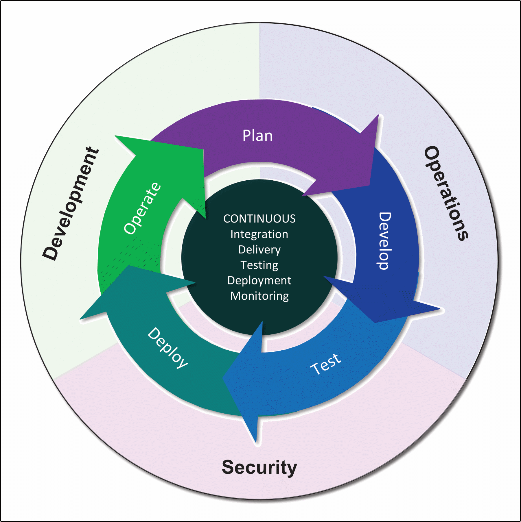
A secure DevOps environment incorporates the tools and processes necessary to protect the application and its data at every stage of the operation. Security starts with the planning and design phases and continues through the entire application lifecycle, baked into the continuous integration and delivery processes. In this sense, security merges with development and operations to create a cohesive three-pronged approach to application delivery, as shown in Figure 1.

Figure 1. Incorporating security into the DevOps process

Secure DevOps calls for a shift left in thinking that pushes security to the beginning of the application delivery pipeline, rather than dangling it out at the end, where it can be the most disruptive to application delivery. Instead, security is built into the planning, development, testing, deployment, and operation phases.

As with other DevOps processes, the goal is to automate security wherever possible, using testing and monitoring to ensure the proper implementation of comprehensive protection policies. In this way, potential risks can be better identified and mitigated early in the development process, while ensuring the continued velocity of the DevOps process.

Implementing secure DevOps starts with a change in mindset toward security and its role in application delivery. Critical to this attitude are support and buy-in from upper management and other stakeholders. Secure DevOps calls for open collaboration, greater transparency, and a shared set of objectives, along with the appropriate use of automation, proper tooling, and advanced application technologies such as infrastructure-as-code.

Secure DevOps, sometimes referred to as DevSecOps, is as much a process as a philosophy, one that sees security as a shared responsibility by everyone involved in application delivery. DevSecOps bridges the gap between development and security teams, helping to reduce the contention that can sometimes occur with traditional approaches to security.

By embedding security processes directly into the application delivery pipeline, DevSecOps offers early and continuous risk management through testing and monitoring, which provide in-depth insights into possible vulnerabilities.

Secure DevOps can also promote a culture of security, encouraging team members to be mindful of the importance of data and application protection at all times. With DevSecOps, developers are more likely to consider security when planning and building applications, QA professionals are more likely to take security risks into account when testing applications, and operation specialists are more likely to adhere to security best practices when deploying application infrastructures.

DevSecOps also leads to more secure and compliant applications because continuous testing and monitoring are integrated into the pipeline at a granular level, making the process more efficient at identifying and limiting threats and compliance violations. With DevSecOps, security becomes a natural part of the application design and fully integrated into the entire delivery process.

Secure DevOps can also make application delivery faster and, as a result, cheaper. Security flaws identified early in the design and development cycles can be addressed much more efficiently than if identified later in the process. As with any bugs, the sooner you find security issues, the quicker and easier they are to fix.

The DevSecOps approach also makes it possible for teams to respond more quickly to changing requirements and circumstances because security is baked in from the start, rather than ladled on top of the application at the end. This integration can also translate to a better user experience, in part because of security is built in, but also because feature updates and application fixes get to users faster.

Implementing secure DevOps

The logistics of integrating security in DevOps will vary from one team to the next, but most teams will follow several basic practices, some of which they might have already incorporated into their infrastructures. For example, in a DevSecOps environment, all source code should be stored in a secure version control repository, leveraging such technologies as encryption and digital signing.

The secure DevOps team should also practice the principle of least privilege so that only authorized individuals can access system resources, with access specific to their job roles. In addition, developers should work with code in small chunks so it’s easier to identify vulnerabilities, and all code should undergo peer reviews, including any scripts used to build infrastructure or deploy applications. The code reviews should look specifically for security risks, compliance violations, and adherence to best security practices.

As with DevOps itself, automation is key to successfully implementing DevSecOps, which requires tools that can seamlessly integrate into the continuous integration and delivery processes. For example, an organization might use Puppet for its automation framework and use Splunk in conjunction with Puppet to provide the analysis necessary to determine when a configuration goes out of compliance. To provide masked copies of databases for development and testing, organizations might use an automated solution like SQL Provision.

An organization might also use a monitoring tool such as WhiteSource, which detects open source components in the code and alerts team members to security risks and software bugs. There are plenty of other tools out there as well, which can help address security throughout all phases of application delivery—and more tools are emerging every day.

Continuous testing is a critical component of automating security, and there are many types of tests that can be performed. For example, DevOps teams might use static application security testing (SAST) to automatically analyze code for security vulnerabilities, without running the application. They might also use dynamic application security testing (DAST) to analyze the application for vulnerabilities when it’s running. Teams might also utilize penetration tests, threat investigations, vulnerability assessments, data flow analytics, and numerous other strategies to help ensure security and compliance.

Just as important as testing is continuous monitoring, which automatically tracks security-related metrics throughout the application delivery lifecycle. The collected information should reflect a wide range of information for identifying security issues. It should also include a system for alerting team members when issues are discovered, such as when code fails a compliance test. In addition, the monitoring solution should offer systemwide information that provides team members with a security overview as well as specifics that might be required for a security or compliance audit.

Moving from DevOps to DevSecOps

Although security might seem at odds with DevOps methodologies at first glance, incorporating security into the DevOps process is an inevitable outcome of today’s sophisticated cyberattacks and expanding privacy regulations.

Organizations that fail to incorporate a DevSecOps mindset are likely to lose ground when trying to implement safe applications that meet the necessary security and compliance standards. For most teams, incorporating security in the early stages of application development is the only viable option in a world of increasing threats, stiffer penalties, and greater risks to the organization’s reputation and the public’s trust.

The post Introduction to DevOps: Security, Privacy, and Compliance appeared first on Simple Talk.


from Simple Talk https://ift.tt/301V5Bz
via