How to Create an Ubuntu PowerShell Development Environment – Part 1

Microsoft has made great effort over the last few years toward multi-platform compatibility. A large part of the IT world runs on Linux. Microsoft recognizes this and has been deploying a lot of their software to now run on the Linux platform. Visual Studio Code, PowerShell, even SQL Server can now run on Linux. As such, it can be beneficial to create your own Linux development environment on your desktop, whether for doing work or just for learning.

While it would be nice to have a computer to install Linux and our other tools directly on, often referred to as a “bare metal” install, most people don’t have extra computers laying around. The solution to this is the use of a virtual machine. In this article, part 1 of 2, I’ll show you how to setup a virtual machine, often referred to as a VM.

Into that VM, you’ll install a Linux distribution, often referred to as a “distro” in the Linux community. It’s important to understand that Linux is the core of the operating system, often called the kernel. Around this kernel people have developed many server and desktop environments. This article will demonstrate use of the most popular ones, Ubuntu, specifically the 19.10 version.

Part 2 of this series will demonstrate how to install PowerShell, Visual Studio Code, and other tools into the Ubuntu VM.

This will create a foundation for a future article, in which you’ll see how to install Docker, then SQL Server into the VM. You’ll then see how to use PowerShell to work with SQL Server as it runs in the Docker container.

VirtualBox

The first thing you need is virtualization software, this is the software that will host and run the virtual machine. Hyper-V is one choice, and if you have it and are comfortable with it, you are welcome to use it for this project.

Hyper-V does require you to have Windows 10 Pro. Many people, especially those at home, may not have the Pro version. For this article then I will be using VirtualBox.

VirtualBox is free, and easy to use. It is also multi-platform, it will run on Windows, Linux, macOS, and Solaris. This article will cover running it on Windows. Do be aware you cannot run VirtualBox and Hyper-V on the same machine, as they both need exclusive access to the same system resources.

You can obtain VirtualBox by going to their website, https://www.virtualbox.org/ and downloading it. Installation is extremely simple, there are almost no options. You can take the defaults for an easy install.

Ubuntu 19.10

After getting VirtualBox installed, you will need a copy of the Ubuntu 19.10 ISO image. The ISO is a file that can be used to install operating systems. ISOs can be written to a USB key or DVD and used to boot a computer, or in this case as a source for VirtualBox.

Getting the ISO is easy, just go to https://ubuntu.com/ . On the front page in the title bar is a Download link. Clicking on it will take you to the downloads page for 19.10, where you will want to download the desktop version of Ubuntu.

From the downloads, simply save the ISO file to your hard drive. Note if you want to experiment with other versions of Ubuntu, simply go to the Downloads link in the upper right and you’ll find other versions you can experiment with.

Creating the Ubuntu Virtual Machine

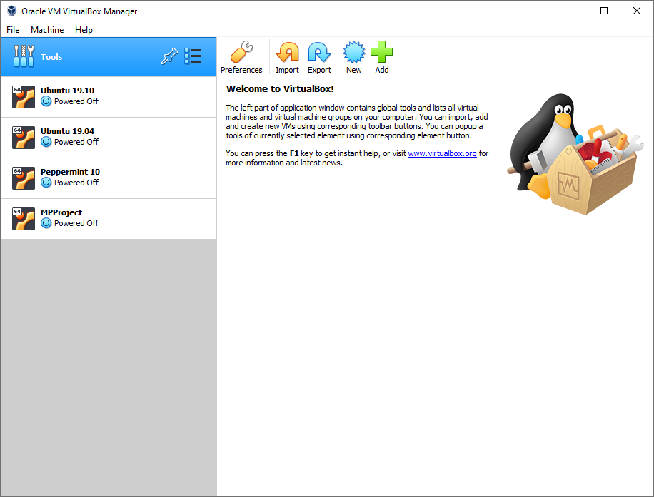
Now you’re ready to take the first step and create the virtual machine. Open VirtualBox, and you’ll see the following screen. In this shot, on the left you will note a list of VMs that I have from other projects, your area will be empty initially but will soon be populated with your own virtual machines.

Setting the VM Name and Type

Start by clicking the big New button in the toolbar to begin the process of creating our VM. When you do, the following dialog in appears. Click Expert Mode to see all the options instead of a wizard.

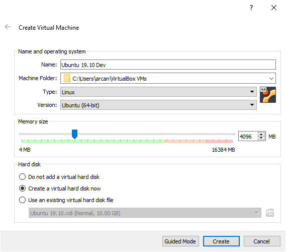
Here you can see I’ve filled out the basic information needed to create the VM. First, I gave it a good name. I took the default for the Machine Folder, that is the path where the virtual machine information will be stored. Note this is for the VM metadata but does not include the location of the virtual hard drive, which will be set in a moment.

I’ve made sure to set the Type to Linux, and the version to Ubuntu (64 bit). The next setting, Memory size, will be somewhat dependent on the computer you are using. Typically for this type of application you want at least 4 gigabytes, or 4096 megabytes, which is what I have set here.

Finally, make sure the Create a virtual hard disk now is selected the click the Create button.

VM Hard Disk Options

On the next screen you are presented with options about the virtual hard drive that will be created. Here is the screen all filled out.

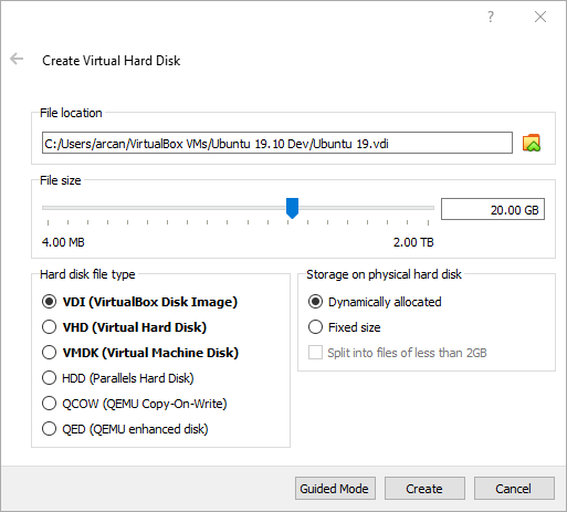
You can store the virtual hard drive in a different location than the rest of the VM’s data. The File location box is used to indicate that location. A helpful hint, often you can get a performance boost by storing your virtual hard drives on a different physical hard drive than the one of the host operating system. Commonly, the operating system running on the computer itself is referred to as the host operating system. Any virtual machines are known as the guest operating system.

Next up is the File size. Because you will be working with SQL Server, you may need extra space, so initially I recommend setting this to 20 GB. You can do so by using the slider bar, or simply typing into the box to the left of the slider.

On the lower left is the file type, and there are multiple choices. VDI is the native type for VirtualBox, and what will be used for this article. However, VirtualBox also supports types may other types from other virtualization software. VHD is the format for Hyper-V, VMDK for VMWare, and so on. Typically, you would not create a full OS drive in another file type, however this capability may be used later to attach files from other virtualization software to read their data.

Finally, on the lower right, you’ll see the Storage on physical hard disk options. With the Dynamically allocated option, VirtualBox will only take as much space as it needs for the drive, up to the maximum indicated in the file size area (in this case, 20 GB). The second option, Fixed size, will create the virtual disk at its maximum size of 20 GB. Fixed size can perform a bit better as it does not need to worry about checking for disk size and expanding on the fly, it also takes up disk space that may not be needed much of the time. For this article go with the dynamic option and click Create.

Setting Additional VM Options

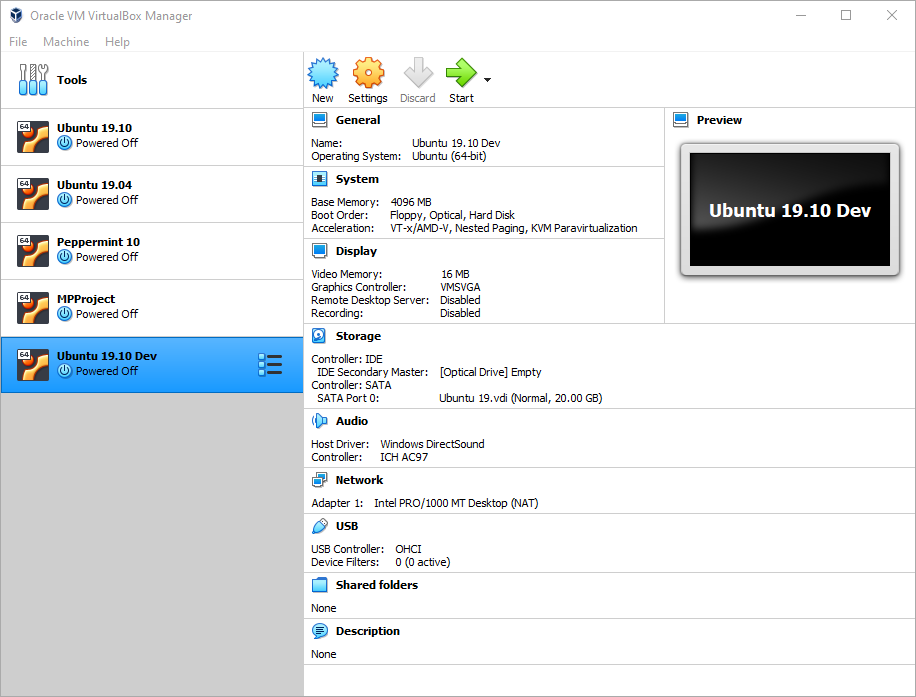
When you create the VM, it now appears in the list on the left. On the right are the machine options.

General Settings

Before you can launch your new VM, there are some settings you need to update. Do note though, if you go into the settings of a running VM many options will be disabled, and this holds true regardless of what virtualization software you are using. You can change the majority of settings only when the VM is shutdown. You won’t have that issue quite yet as you haven’t installed Ubuntu in the VM yet, but it’s something to be aware of for your future use.

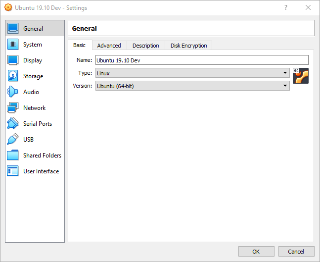
Start by clicking on the gold Settings gear icon in the toolbar. As you can see, the dialog that appears allows you to change many options.

While still on the General settings page, click on the Advanced tab.

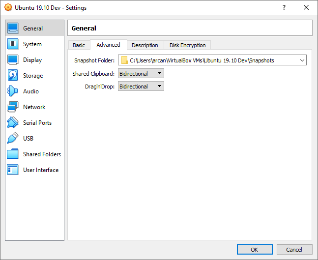
On this tab, change the Shared Clipboard and Drag’n’Drop to Bidirectional, as you see above. This will allow you to cut and paste to and from the virtual machine. Likewise, you can copy files into the VM using drag and drop. This is entirely optional, of course, but will make it much easier to work with the VM. Do note that if you are doing security testing of some type, you will wish to alter these settings to either Disabled, or just allow pasting into the VM by picking Host to Guest. However, this is a simple development box so having bidirectional copy/paste will be fine.

System Settings

Next, click on the System page on the left to bring up the system settings.

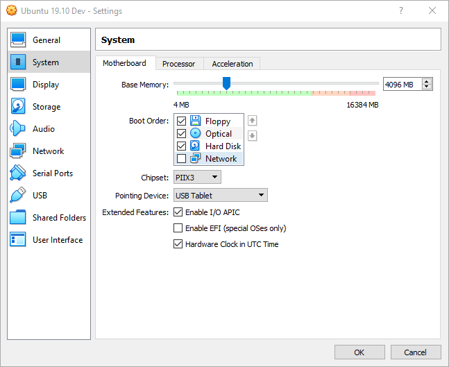
The first tab is the Motherboard; it is on this page where you can change the amount of ram for example. Don’t change anything on this tab, but it very useful to know where to come should you later decide you need to change the amount of ram or any of the other motherboard settings. Take a look at the Processor tab next.

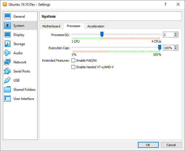
By default, VirtualBox set up this VM with 1 CPU. The computer I’m writing this on has 4 CPUs, so I have opted to increase the CPU count to 2, as you see in the above image. Ultimately this is something you’ll have to determine based on the physical characteristics of your host computer, as well as the demands you’ll be placing on the VM. In my case, I only plan to run one VM at a time, and I won’t be using many resources in the host computer while I am working in the virtual machine.

Now it’s time to move on; click on the Display option on the left.

Display Settings

There are a few changes on the Screen tab you should make here to increase performance.

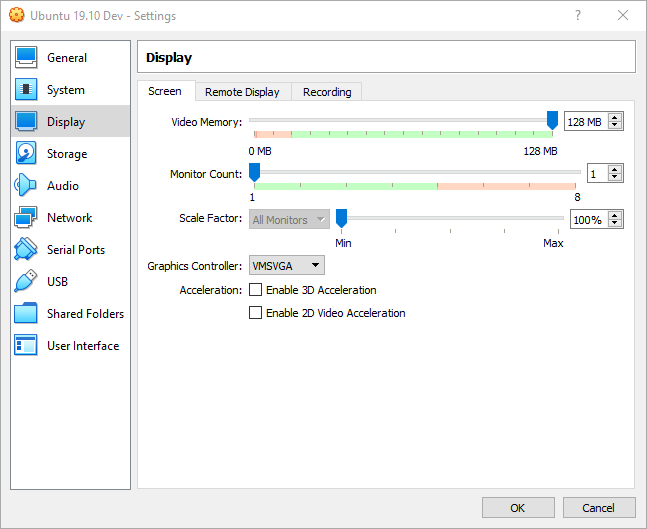
First is the Video Memory. By default, it is at 16MB. I suggest maxing it out to the full 128MB. If you discover later this provides too negative of an impact to your system you can always adjust it to a lower value.

I want to call your attention to the next item, Monitor Count. VirtualBox will let you create multiple virtual monitors, a very helpful utility when you have multiple physical monitors on your host computer. When I first setup a new virtual machine, I always leave this to 1, as you see here. Once I have the VM up and running, I can return here later and add monitors if needed. For example, at home with my laptop hooked to its docking station, I will open the settings and adjust this to 3. Later, when I take my laptop out of the house, I will adjust this back down to 1.

Scaling Factor works just like it does in Windows, it will magnify certain graphical elements in the guest operating system while leaving the resolution alone. I typically leave this set to the default.

The last item of note is the Graphics Controller. We suggest you set to VMSVGA. This setting should allow you to resize the window of your VM, and the VM will then adjust its resolution to fit that of the resized window. However, not all graphics cards respond the same, so you may need to return later and try some of the other settings. Once a virtual machine is created, you can easily go back later and edit things like the graphics controller.

Also be aware some guest operating systems may not support this feature, although the Ubuntu 19.10 used in this article does.

There is one last thing to update, and it is the most important to getting our VM up and running. Click on the Storage icon on the left.

Storage Settings

In order to install the Ubuntu, you need to insert the Ubuntu ISO image into the VM’s virtual CD/DVD drive. It is in this step you will accomplish this.

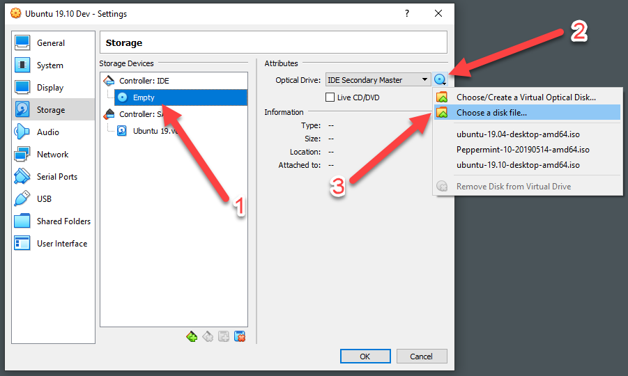
Start by clicking on the Empty label, pointed to by number 1 in the above image.

To the right of the Optical Drive is an icon of a DVD (pointed at by number 2). Click on it to expand the menu.

Now click on Choose a disk file…, indicated by number 3 in the above graphic. Note that if you have installed other VMs in the past, the most recent three ISOs used will appear in the menu. If one of these is the operating system you want to install, you can simply pick it. In this case, navigate to the ISO you downloaded from the Ubuntu site.

Other Settings

There are no more modifications to make in order to proceed. You are free of course to explore the other setting pages. I do want to call your attention to the Shared Folders page. With Shared Folders, you designate a folder location in your host operating system. That folder will then appear inside the file manager inside your guest operating system. This makes it very easy to copy files in and out of your virtual machine.

Just click the big OK button to save your configuration settings and proceed to the next step.

Installing Ubuntu 19.04

Now that you have the machine configured it’s time to get started installing Ubuntu. Make sure the new Ubuntu 19.10 Dev VM is selected in the list of VMs on the left, then click the green Start arrow in the toolbar above the VM settings.

If you forgot to attach the ISO in the previous step, when the machine launches, VirtualBox detects there is no operating system installed. Here it is prompting you for the ISO image to use.

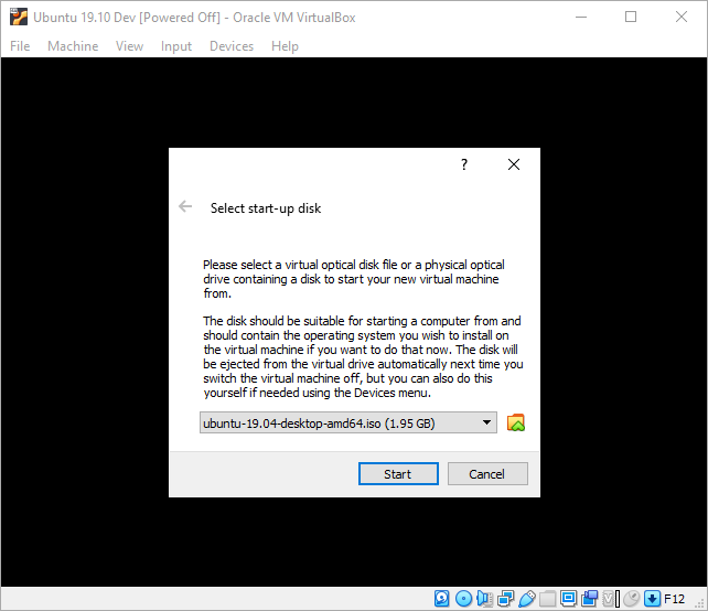
If you remembered to connect it, you’ll skip the above screen. It’s a common mistake to miss attaching the ISO so we wanted to make sure to mention it.

Because you had loaded the Ubuntu ISO in the Storage settings in the previous section, it defaults to it. Just click Start to run the machine with this ISO.

If you are running on a slower machine, you may see the following dialog.

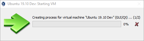
At this point VirtualBox has begun the processes of setting up the VM. Just sit back and wait. The amount of time it will take depends on your computer, so be patient. If you computer is fast enough, you may not see the above dialog box at all.

You will soon see a new window open, with the Ubuntu Virtual Machine. It will take it a little time to spin up, don’t be surprised if you see a blank screen for a little bit. Eventually you will see the Ubuntu installer appear.

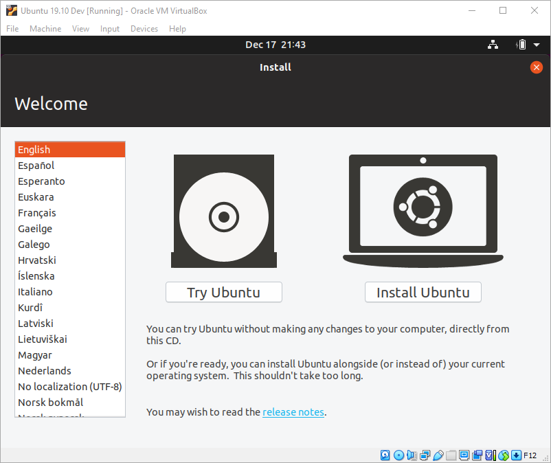
Here you have two choices, Try Ubuntu or Install Ubutnu. Ubuntu is distributed as a Live DVD. In Live mode, you could use a tool to create a bootable USB stick, then boot your physical computer to the USB stick instead of your hard drive. Using the Try option would let you experiment with Ubuntu without making changes to your computer. (If you decide you want to try this for yourself, I recommend the balenaEtcher tool, available at https://www.balena.io/etcher/ ).

In this case you are installing in a virtual machine, with no risk to the host operating system, so after verifying the correct language is selected on the left, click the Install Ubuntu option.

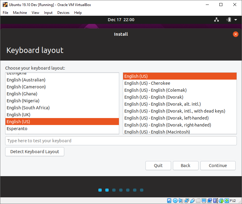
The first thing you are asked is to confirm your keyboard layout. Ubuntu does a good job of figuring it out and picking it automatically, but if you would like to pick something different this is the time to change it. If you are happy, then just click the Continue button.

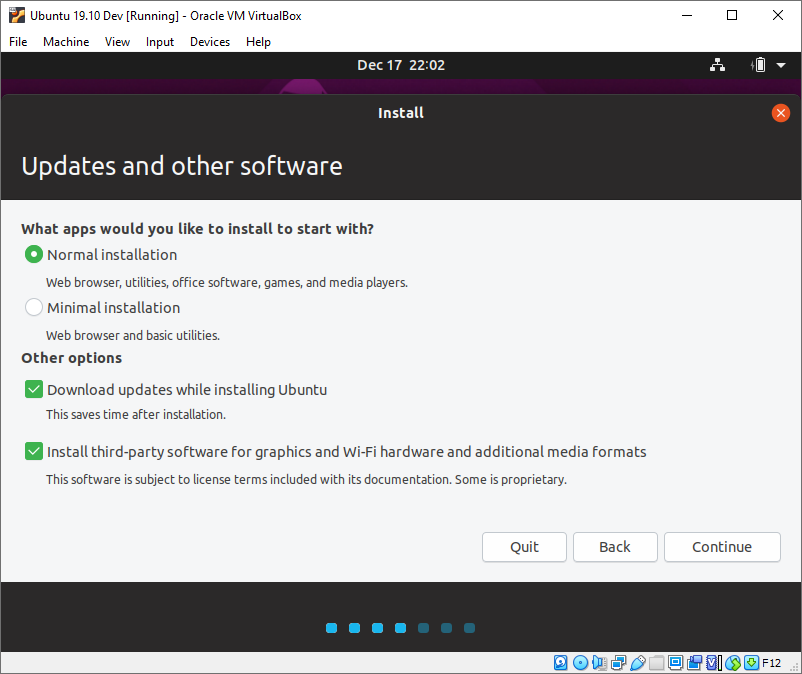
In the next screen, you are given some options. First, it wants to know if you want a normal install or minimal. With minimal, only the web browser and a few basic tools are installed. In normal mode, it will also install office software, media players, and more. I suggest using the Normal Installation option, as it’s often useful to have some of the office tools in your VM. Don’t worry though, if you go with a minimal install, you can easily install other things from the Ubuntu software store that is built into the Ubuntu operating system.

Under the other options, the Download updates… is checked on by default. While you can install updates after installation, it makes it easy to just go ahead and download them now. It will add a bit of time to the setup operation, but if you have a decent internet connection this will be minimal.

The last option, Install third-party software… is unchecked by default. Some Linux users are “purists” and will only use open source software. Others are more pragmatic and are willing to use software that may be closed source or proprietary, such as video and other hardware drivers. I personally fall into the “pragmatic” camp and check this on, as I’ve done here. This is a choice you will have to make, but for this article I suggest checking it on as shown in the above image and click Continue.

In the next step, you are asked about the installation type. Since the virtual disk is empty, go with the default option of Erase disk and install Ubuntu. The other options are geared toward installation on a physical computer, or into a machine that you want to install Ubuntu side by side with another operating system.

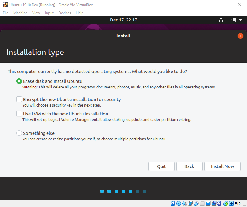
At this point you are ready to begin the installation, so simply click the Install Now button. Because you picked the erase disk option, you are given a warning that you are about to create changes to the target drive.

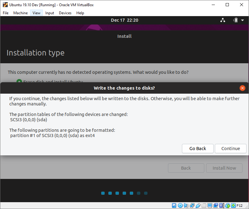
This is OK, it’s what you want, so just click the Continue button.

Next, you are asked what time zone you are in. VirtualBox will provide the current date/time info from the host operating system to Ubuntu, and it will default to that time zone. If you need to use another time zone though, this is a good time to change it.

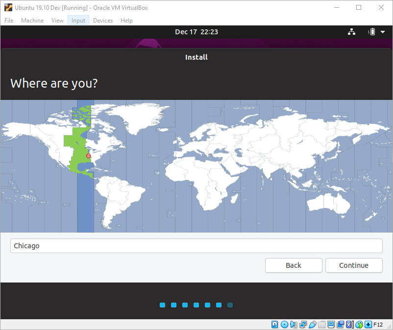
In my case, I am in the Chicago (Central US) time zone, so I will just click Continue.

In this next screen, you are asked for some information about your user ID in this virtual machine. Your name is up to you. Typically, you might enter your full name, such as Robert Cain. When it comes to VMs though, I generally use the same information here as my username. For the computer name, I usually begin my virtual machines with vm- in case I am using a network tool. It will be clear this is one of my virtual machines and not a physical computer. After this I’ve added the same information as the name it was given in VirtualBox.

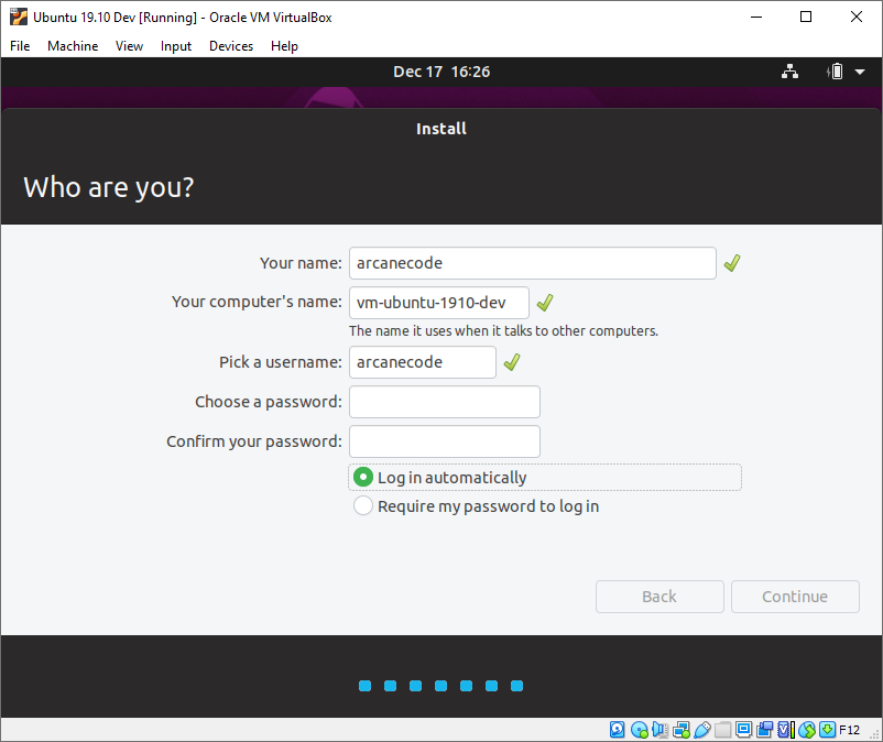
Next up is the username, this is a choice for you to make. Below it you will enter the password to use. Be aware this password is used for more than just logging in. Whenever you install software or alter other system settings, Ubuntu will prompt you for this password as a security measure, to confirm you have permission to make these changes. As a result, you should select a password that is complex enough to be secure, but easy to type and remember as you will be entering it a lot. Note in the above image I haven’t entered the password, when you do it will appear as dots. After entering a password you’ll need to re-enter it in the confirmation box.

The last option is in regard to logging in. The default will be Require my password to login. If you are installing Ubuntu on a physical computer, or in a user testing / production situation, then I highly advise taking this option. In this case, you are creating a machine for simple development and learning so you might want to change it Log in automatically. If this makes you uncomfortable or violates a corporate policy, then by all means go with the default.

Once you are ready, click Continue.

At this point Ubuntu begins installing.

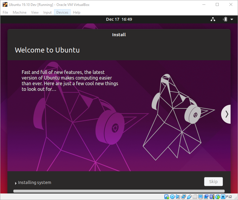
Here you see the progress bar. As it proceeds you will see the display update with helpful tips and tricks. Take a look at them as the install proceeds, it includes some helpful information.

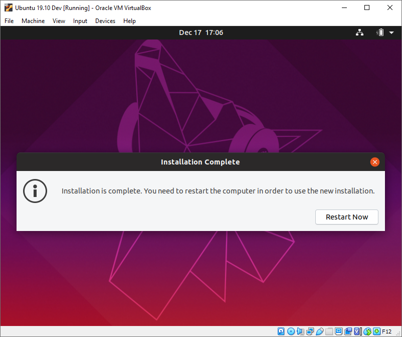
When the installation completes, you will be prompted to restart. Simply click the Restart Now button.

After it reboots, you will be prompted to remove the installation medium then press Enter.

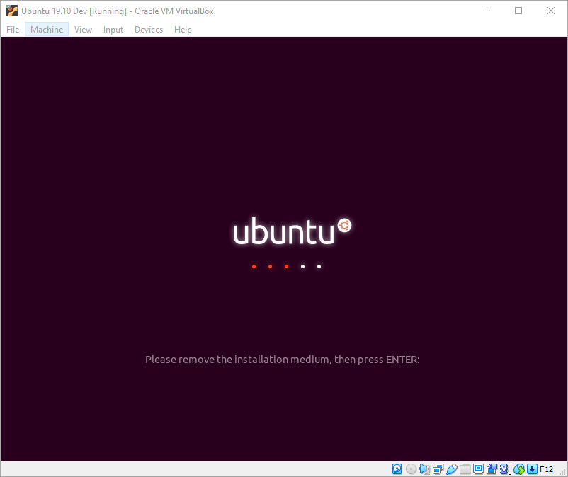
In this case VirtualBox has already taken care of this for you, so all you have to do is click the mouse inside the VM window (so it gets the focus) and press the Enter key.

Once Ubuntu restarts again, you will be prompted to connect your online accounts.

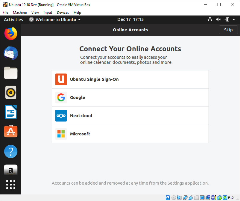
Since this is a virtual machine for doing development, I usually skip this step by clicking the Skip button in the upper right.

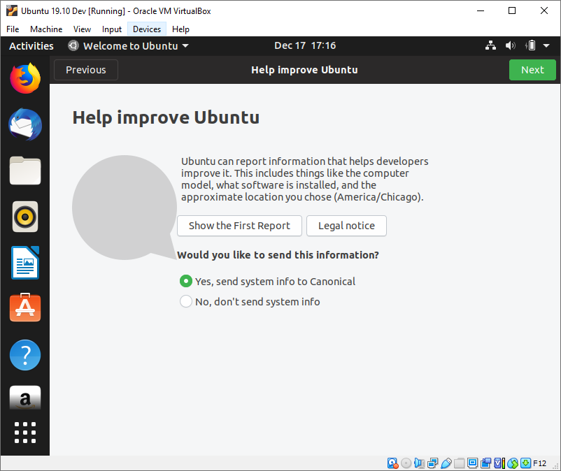
In the next step you are prompted to send system reports to Canonical, the makers of Ubuntu. I usually leave this at the default, but some companies have policies that state you should not share this information. Other people are not comfortable with sharing, so take which ever option you wish and click the Next button in the upper right.

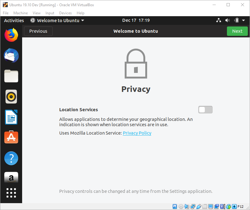
Next Ubuntu wants to know if it can activate Location services. These services are used for things like mapping websites, or when you go to an online store. By default, it is off, and as this isn’t overly useful in a virtual machine (unless you are developing software that needs these services) just take the default and click Next.

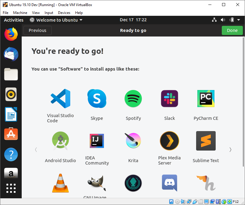
Finally, you’re done! You’ve installed and configured your Ubuntu VM. You can now click Done to close out the window and begin the next steps, updating Ubuntu and installing the software you’ll need.

Updating Ubuntu

In the next article, I’ll go through the process of installing PowerShell, Visual Studio Code (also known as VSCode), and Azure Data Studio. Before that, there are some updates as well as install a few small utilities that will make life easier. You may not use all of them in the next few articles, but as you move forward with your Linux experience, they will become handy to have.

The first thing you’ll find is Ubuntu has a very low timeout before it goes into lock screen mode. In my opinion, when running as a virtual machine, this is unnecessary. Your host system should be set to lock automatically after a set time, or when you choose to lock it manually. Having your virtual machine auto lock as well can get annoying. This first step is optional, but I think you’ll find the short timeout annoying as well, so here’s how to disable it, or if you prefer to extend the time before the VM auto locks.

In the upper right corner, next to the battery icon, is a drop-down arrow. Clicking it will bring up a menu.

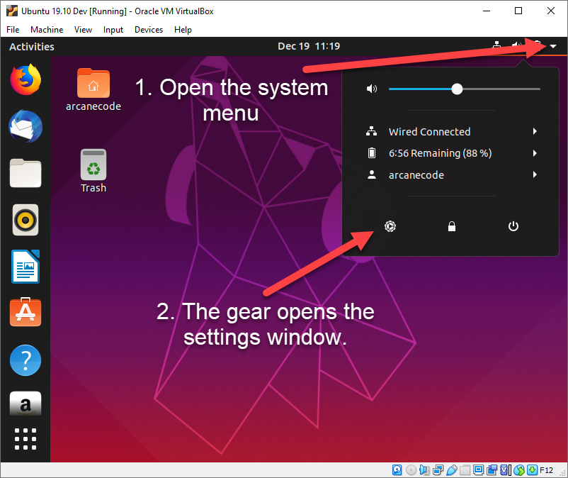
In the menu, click on the gear icon to bring up the settings window. If you are new to Ubuntu, I’ll mention a few other things. The lock icon in the middle will lock your virtual machine. Getting your machine out of the lock state is a bit odd in that you have to press a key on the keyboard to bring up the password entry dialog. Mouse clicking has no effect.

Next to the lock is the power button, which will give you options to shut down, reboot, and so on.

Go ahead and click on the gear. The settings window will now appear. On the left side is a list of settings categories. Scroll down and click on the Power settings.

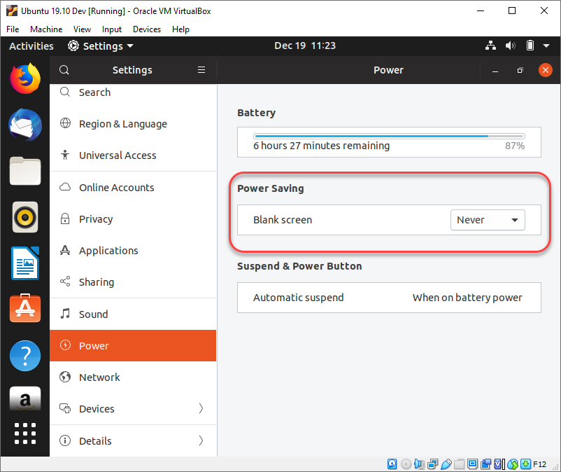
In the middle is the Power Saving area (highlighted by the orange rectangle in the above graphic). Use the drop-down to change the setting to Never, or to another setting you are comfortable with. There’s no need to press any kind of a save button; when you make a change Ubuntu automatically applies it. Just click the orange X in the upper right corner to close this window.

Opening the Terminal

Now that you VM won’t time out on you, you’ll do a general update to Ubuntu itself. You’ll be doing a lot of this through the terminal, so go ahead and open a terminal window. The 9 dot grid in the bottom left of the Ubuntu desktop is similar to the start menu in Windows. Click on it to bring up your installed applications.

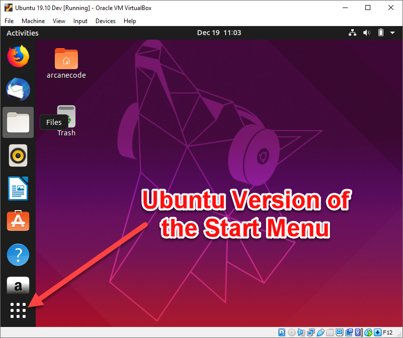
After clicking on the “start menu” the screen updates to show all your apps.

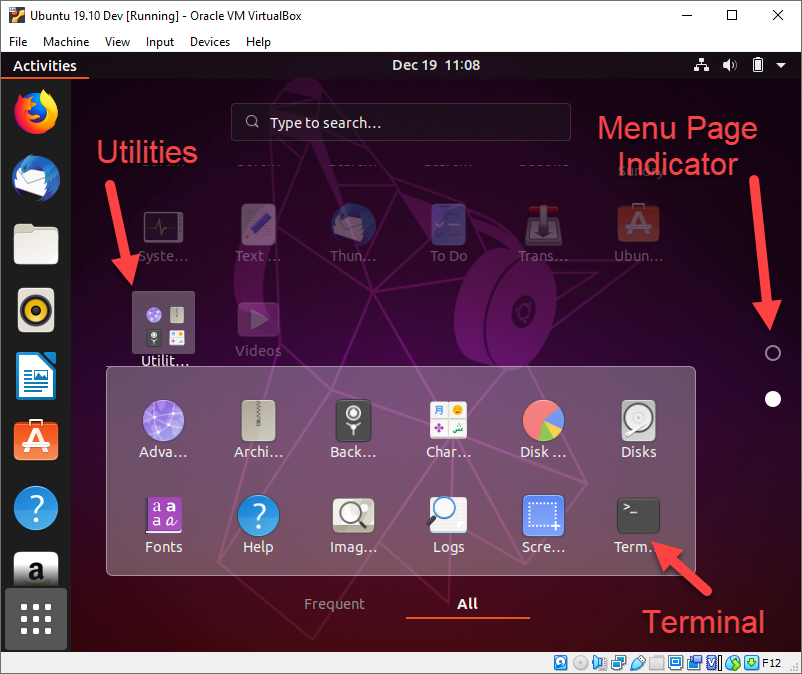
Over to the right is the Menu Page Indicator. The number of menu pages is dependent upon how many applications you have installed and the size of your screen. In the above screenshot the Menu Page Indicator shows I have two pages of menus; there will be a dot for each page and the solid dot indicates I am on the second page.

To get to the terminal, find the box labeled Utilities. This is a submenu, when you click on it the Utilities expands, and in it you’ll find the icon for the Terminal.

There is a second method for getting to the terminal that you could use. Many Linux distros have a built-in keyboard shortcut to launch the terminal, in Ubuntu CTRL+ALT+T will launch a new terminal window. Other distros use the Superkey+T shortcut, where superkey would be the Windows key on many keyboards. No matter which way you choose, it’s now time to open up a terminal window and continue our setup of Ubuntu.

Apply Updates

Before proceeding, you should first apply any new updates. Doing so is very easy, at the terminal window enter the following command.

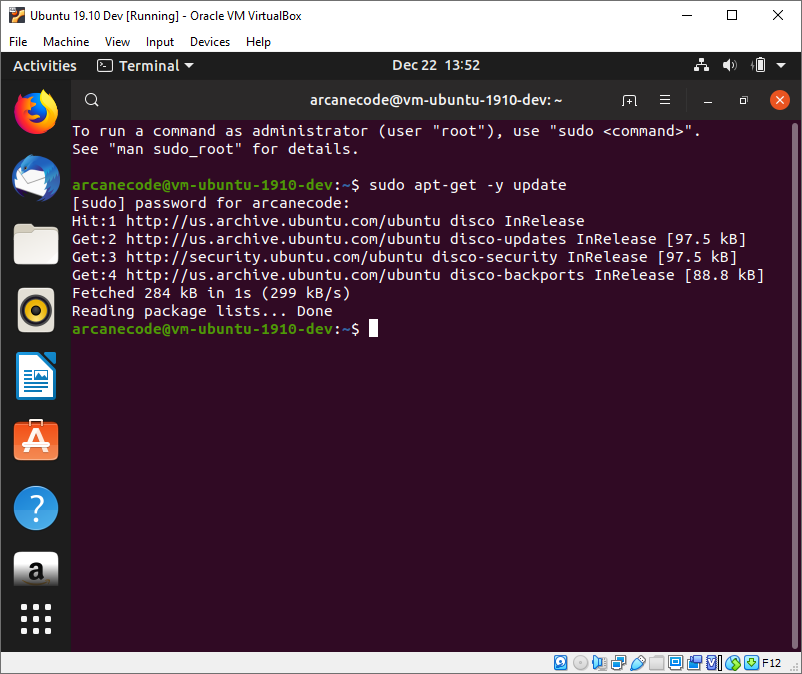
sudo apt-get -y update

The sudo command is short for Super User DO; it is the equivalent of “Run as Administrator” in Windows. When you enter a command using sudo you’ll be prompted for your password. If you enter more sudo commands, Linux will remember your recently entered password for a brief time so you don’t have to keep reentering it.

The apt in apt-get stands for Advanced Package Tool. It, as well as the apt command you’ll see in a moment, is part of a suite of tools used to install new applications or keep your system up to date. In order to understand how this works, you need to understand how Linux manages packages. Each Linux distro maintains its own set of package repositories. Think of it as a sophisticated lookup tool. When you issue an apt command to go get application “X”, your operating system looks in its library for “X”. It has an entry to go to a specific location on the internet, where application “X” can be downloaded, along with any special instructions for installation. Note the apt commands can also be used for more than just applications. It may also be used to install operating system updates, as in the above example, or to upgrade your operating system to a more recent version.

It is also possible to add additional repositories to your distro. Many companies provide their own set of package repositories with which you can use the apt commands to install and update their specific applications.

Returning to the syntax of the command, the -y tells the apt-get command to automatically reply yes to any “are you sure” style prompts. Finally, the update tells apt-get to make sure all operating system components and applications are up to date.

Now that you understand the basic syntax of the command, enter it and press enter. You’ll be prompted to enter your password, do so and the update process will begin.

Install Additional Utilities

There are a few utilities that you may need as you work with Ubuntu over time. While you won’t necessarily use these during this course of articles, they are common to many developer installs. As you read through other tutorials here on Red Gate’s Simple Talk site as well as other locations, it will be assumed you have these already installed. As such, I go ahead and install these as part of my developer installs and suggest you do so, too.

VIM

First, install a basic text editor called VIM. VIM works in the terminal and makes it easy to edit text files. To do so, use the apt command just discussed.

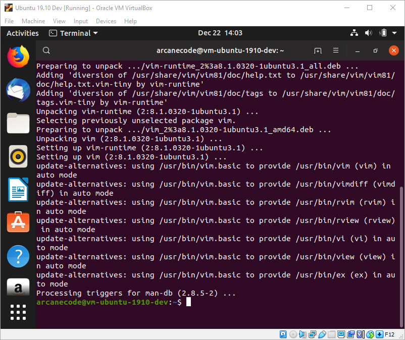
sudo apt -y install vim

Note this code is using only the apt command, not apt-get. It’s also using install to indicate you are installing a new application, and vim is the name of the application to install.

This would be an opportune time to mention that Linux is case sensitive. If I had used VIM instead of vim in the above example, the apt command would have failed.

This also applies to file and directory names. For example, myfilename.txt, MYFILENAME.TXT, and MyFileName.txt refer to three different files, and all three could exist in the same folder.

net-tools

Having a set of network tools can be handy to do things such as discover your network status and information. Those are found in a suite of tools called net-tools. To install, use the following command.

sudo apt -y install net-tools

Once it has installed, you can use the command ifconfig to test it, ifconfig will display your network configuration.

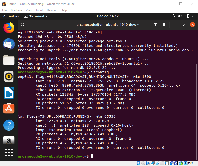
As you can see, ifconfig returns quite a bit of useful information about our machine’s network info.

Git

Many developers use a code repository to store the source code to their applications. A code repository is a bit different than the Linux repositories you’ve seen so far in this article. Those repositories are used to hold installable applications. The git repositories are used to hold the source code needed to build those applications.

Git is one flavor of a repository. It can be hosted locally, within your own company, or on a platform. GitHub is probably the most popular of these and can host both public and private repositories for free. As it is used so much, I go ahead and install in every developer system I set up.

sudo apt -y install git-all

By now most of this command should be familiar to you, git-all is the application name that will install all the git components.

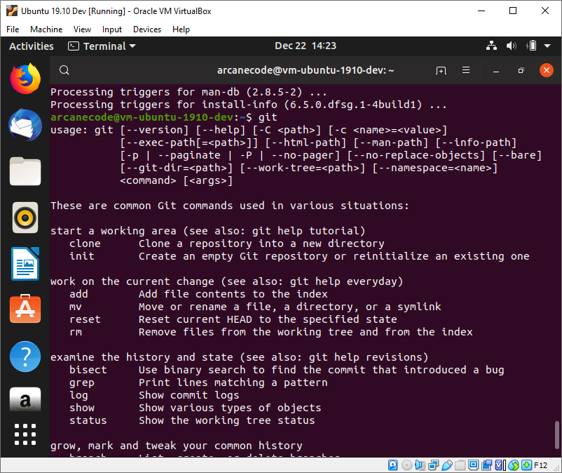
Once installed, you can enter the command git to confirm it was installed. It will show you the basic help for the git application.

Snap

The apt command is not the only method by which you can download and install applications. The two most popular in the Linux community are flatpacks and snaps. Ubuntu favors the snap method, and the most recent versions of Ubuntu already have the snap application installed. To see if you have it, simply enter the command snap in the terminal and press enter.

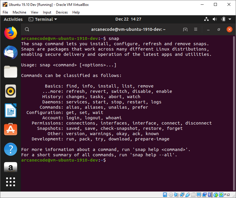
Should you get the error message that snap was not found, you can install it by using apt.

sudo apt -y install snapd

Two things to note, first that is not a misspelling in the command, snapd is the name of the application to use. Second, snaps are only supported on Ubuntu versions 18.04 and later.

Conclusion

This article covered the first steps in setting up a development environment for developing PowerShell Core scripts in a Linux environment, specifically Ubuntu. It described using VirtualBox as the virtual machine manager, downloaded Ubuntu, and configured VirtualBox for a new Ubuntu install. With minor modifications, you could have also adopted the instructions for Hyper-V, or set up an empty PC with Ubuntu running “bare metal”, right on the computer itself.

It then covered installing Ubuntu 19.10, stepping through each screen in the installation process and discussing the options, allowing for choices when installing in a virtual machine versus a real computer. After installing, you logged in, updated Ubuntu, and then added several small utilities such as VIM and the networking tools.

In part 2 of this series, I’ll demonstrate installing PowerShell Core and Visual Studio Code. In addition, you will learn how to install Azure Data Studio to prepare for future database work. I’ll wrap up part 2 by automating the update to the favorites bar, configuring it for a development centric environment.

This foundation is a good position for growth. I’ll expand on the base created in parts 1 and 2 in future articles, including one on installing SQL Server in a Docker container on Linux.

The post How to Create an Ubuntu PowerShell Development Environment – Part 1 appeared first on Simple Talk.

from Simple Talk https://ift.tt/2ugK2um
via

Efficient Solutions to Gaps and Islands Challenges

Gaps and islands analysis supplies a mechanism to group data organically in ways that a standard GROUP BY cannot provide. Once we know how to perform an analysis and group data into islands, we can extend this into the realm of real data.

For all code examples in this article, we will use a set of baseball data that I’ve created and maintained over the years. This data is ideal for analytics as it is large and contains data quality that varies between very accurate and very sloppy. As a result, we are forced to consider data quality in our work, as well as scrutinize boundary conditions for correctness. This data will be used without much introduction as we will only reference two tables, and each is relatively straightforward.

Once introduced, we can obtain metrics that may seem challenging to crunch normally, but by using a familiar and reusable gaps/islands algorithm, we can make it (almost) as easy as cut & paste.

Gaps and Islands: Definitions and Data Intro

Our first task is to define a programmatic way to locate gaps and islands within any set of data. To do so, consider what a boundary is within different data types:

• For a sequence of integers, a boundary can surround missing values.
• For dates/times, a boundary can represent the start or end of a sequence of frequent events that are chronologically close together.
• For decimals, boundaries may be defined by values that are within a small range of each other.
• For strings, missing letters or letter sequences may define a boundary.

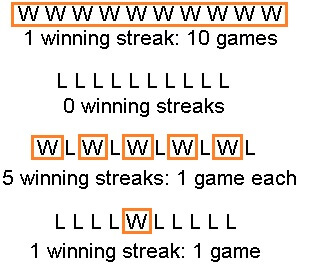
These represent a starting point for considering ways to slice up data. A critical aspect of this work is that the result set of gaps/islands analysis will vary in size. For example, if we wanted to measure the number of winning streaks by a sports team as a data island, then there could be any number from zero to (N + 1) / 2 islands, given a set of N rows. This assumes a repeating sequence of winning and losing “streaks” of one game each.

The following diagram shows a set of 10 win/loss events and different ways that islands of data could look:

The image illustrates result sets of 0, 1, and 5 rows for island counts. Note that a single winning streak of 1 game and a single winning streak of 10 games each result in a single identifiable island of data. The key here is that if we are generating a dataset of winning streaks, the result set will vary in size based on the underlying data.

Let’s jump into baseball data and crunch winning streaks as islands of wins and losing streaks as islands of losses. Conceptually, islands are easier to manage and understand than gaps. This convention also allows us to write all our queries similarly, regardless of the results we are seeking.

Here is a sample of the data we will be working with:

SELECT TOP 10
        *
FROM dbo.GameLog;

The results show a row per game with a sample of metrics, including team names (abbreviations), game date, score, and more. GameNumber indicates if a game was part of a double-header so that we know the order of games within a given day, when applicable. The details continue for many more columns and tell us who played each position, the umpires, and totals for many metrics within the game. For the sake of our work, the most basic high-level details are all we will need.

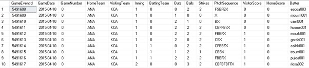
We will use an additional table that contains play-by-play details for each game. The following is a sample of that detail:

SELECT TOP 10
        *
FROM dbo.GameEvent;

This table contains a row per play per game. A play is usually an at-bat, but may also consist of an error, stolen base, or other action that can be taken during a game. A single game could have over a hundred events associated with it. Like GameLog, the detail can get exhaustive, but we will focus on high-level, easy-to-understand metrics.

This data contains 219,832 games spanning from 1871 through 2018. There is a total of 12,507,920 events associated with those games. With the data introduced, let’s define a winning streak as a set of wins bounded by losses or ties. With that simple definition in mind, we can dive in and crunch our data.

Gaps and Islands: Calculating Streaks

The simplest analysis we can perform is to determine winning and losing streaks. From a data perspective, streaks can be described as islands of wins or losses. To code this, we need to formulate a reliable and repeatable process so that we are not writing new code over and over for each query. The following steps through what we need to accomplish to complete this analysis.

1. Gather a dataset

No metrics can be crunched without a candidate dataset that provides everything we want without noise or distractions. For baseball data, we will be creating a set of games. For example, if we wanted to find regular-season winning streaks for the New York Yankees, we would need to pull every regular-season game that they played in:

SELECT
   CASE WHEN (HomeScore > VisitingScore AND HomeTeamName = 'NYA') 
          OR (VisitingScore > HomeScore AND VisitingTeamName = 'NYA') 
          THEN 'W'
        WHEN (HomeScore > VisitingScore AND VisitingTeamName = 'NYA') 
          OR (VisitingScore > HomeScore AND HomeTeamName = 'NYA') 
          THEN 'L'
        WHEN VisitingScore = HomeScore THEN 'T'
    END AS result,
    GameLog.GameDate,
    GameLog.GameLogId
FROM dbo.GameLog
WHERE GameLog.HomeTeamName = 'NYA' OR GameLog.VisitingTeamName = 'NYA'
AND GameLog.GameType = 'REG';

Here, we filter on any game where the home team or away team was the Yankees (NYA). We then filter to include only regular-season games (REG). GameLogId is an identity primary key and is used to ensure each row is unique and ordered chronologically.

Lastly, we compare the home and away scores to determine if the game was a win, loss or tie as follows:

• If the Yankees are the home team and the home score is greater than the visiting score, then it is a win.
• If the Yankees are the visiting team and the visiting score is greater than the home score, then it is a win.
• If the Yankees are the home team and the home score is less than the visiting score, then it is a loss.
• If the Yankees are the visiting team and the visiting score is less than the home score, then it is a loss.
• If the scores are the same, then it is a tie. This is uncommon but has happened enough times to be statistically significant.

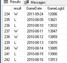
The results are a narrow dataset that lists every game the Yankees have ever played, as well as the result:

2. Determine the Start and End of Streaks

We now want to look at the data above and identify the dates that every winning streak began and ended. To do this, we need insight into the next and previous games. A winning streak begins when a win is preceded by a game that is not a win. A winning streak ends when a win is followed by a game that is not a win.

The easiest way to accomplish this is to use LEAD and LAG on each game to return whether the previous and next games were wins, losses, or ties:

SELECT
    CASE WHEN (HomeScore > VisitingScore AND HomeTeamName = 'NYA') 
            OR (VisitingScore > HomeScore AND VisitingTeamName = 'NYA') 
            THEN 'W'
         WHEN (HomeScore > VisitingScore AND VisitingTeamName = 'NYA') 
            OR (VisitingScore > HomeScore AND HomeTeamName = 'NYA') 
            THEN 'L'
         WHEN VisitingScore = HomeScore THEN 'T'
    END AS result,
    LAG(CASE 
       WHEN (HomeScore > VisitingScore AND HomeTeamName = 'NYA') 
         OR (VisitingScore > HomeScore AND VisitingTeamName = 'NYA') 
         THEN 'W'
       WHEN (HomeScore > VisitingScore AND VisitingTeamName = 'NYA') 
         OR (VisitingScore > HomeScore AND HomeTeamName = 'NYA') 
         THEN 'L'
       WHEN VisitingScore = HomeScore THEN 'T' END) 
         OVER (ORDER BY GameLog.GameDate, GameLog.GameLogId) 
      AS previous_game_result,
    LEAD(CASE 
           WHEN (HomeScore > VisitingScore AND HomeTeamName = 'NYA') 
             OR (VisitingScore > HomeScore AND VisitingTeamName = 'NYA')
             THEN 'W'
           WHEN (HomeScore > VisitingScore AND VisitingTeamName = 'NYA') 
             OR (VisitingScore > HomeScore AND HomeTeamName = 'NYA') 
             THEN 'L'
           WHEN VisitingScore = HomeScore THEN 'T' END) 
             OVER (ORDER BY GameLog.GameDate, GameLog.GameLogId)
        AS next_game_result,
    ROW_NUMBER() OVER (ORDER BY GameLog.GameDate, GameLog.GameLogId) 
        AS island_location,
    GameLog.GameDate,
    GameLog.GameLogId
FROM dbo.GameLog
WHERE GameLog.HomeTeamName = 'NYA' 
    OR GameLog.VisitingTeamName = 'NYA'
    AND GameLog.GameType = 'REG';

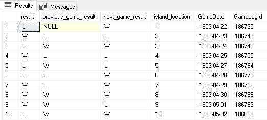
Note that the contents of the result field are copied verbatim into a LEAD and LAG statement. Each are ordered by the game date and ID columns, ensuring chronological order and no chance of ties. Window functions operate over a window (set of rows) and here we are defining the window as the entire dataset with this particular ordering.

In addition, a column was added with a ROW_NUMBER, which numbers every game in order. This allows for some additional math later, such as streak length:

Note that the previous game result is NULL for the first row. Similarly, the next game result will be NULL for the last row in the dataset.

With this work out of the way, we can now identify the start and end of streaks. A critically important mathematical note on this data is that the number of starting and ending data points will always be equal. If we find 100 winning streaks, we know that there will be 100 starting points, 100 ending points, and all 100 of each can join together in order to provide a full dataset.

To find the beginning and end of each streak, we will encapsulate the code above in a CTE and query it accordingly:

--CTE only, doesn’t run
WITH GAME_LOG AS (
SELECT
    CASE WHEN (HomeScore > VisitingScore AND HomeTeamName = 'NYA') 
           OR (VisitingScore > HomeScore AND VisitingTeamName = 'NYA') 
           THEN 'W'
        WHEN (HomeScore > VisitingScore AND VisitingTeamName = 'NYA') 
           OR (VisitingScore > HomeScore AND HomeTeamName = 'NYA') 
           THEN 'L'
        WHEN VisitingScore = HomeScore THEN 'T'
    END AS result,
    LAG(CASE WHEN (HomeScore > VisitingScore AND HomeTeamName = 'NYA') 
           OR (VisitingScore > HomeScore AND VisitingTeamName = 'NYA') 
           THEN 'W'
        WHEN (HomeScore > VisitingScore AND VisitingTeamName = 'NYA') 
           OR (VisitingScore > HomeScore AND HomeTeamName = 'NYA') 
           THEN 'L'
        WHEN VisitingScore = HomeScore THEN 'T' END) 
           OVER (ORDER BY GameLog.GameDate, GameLog.GameLogId) 
        AS previous_game_result,
    LEAD(CASE 
         WHEN (HomeScore > VisitingScore AND HomeTeamName = 'NYA') 
             OR (VisitingScore > HomeScore AND VisitingTeamName = 'NYA') 
             THEN 'W'
        WHEN (HomeScore > VisitingScore AND VisitingTeamName = 'NYA') 
           OR (VisitingScore > HomeScore AND HomeTeamName = 'NYA') 
           THEN 'L'
        WHEN VisitingScore = HomeScore THEN 'T' END) 
           OVER (ORDER BY GameLog.GameDate, GameLog.GameLogId) 
        AS next_game_result,
    ROW_NUMBER() OVER (ORDER BY GameLog.GameDate, GameLog.GameLogId) 
        AS island_location,
    GameLog.GameDate,
    GameLog.GameLogId
FROM dbo.GameLog
WHERE GameLog.HomeTeamName = 'NYA' OR GameLog.VisitingTeamName = 'NYA'
    AND GameLog.GameType = 'REG'),
CTE_ISLAND_START AS (
SELECT
    ROW_NUMBER() OVER (ORDER BY GAME_LOG.GameDate, GAME_LOG.GameLogId) 
        AS island_number,
    GAME_LOG.GameDate AS island_start_time,
    GAME_LOG.island_location AS island_start_location
FROM GAME_LOG
WHERE GAME_LOG.result = 'W'
    AND (GAME_LOG.previous_game_result <> 'W' 
         OR GAME_LOG.previous_game_result IS NULL)),
CTE_ISLAND_END AS (
SELECT
    ROW_NUMBER() OVER (ORDER BY GAME_LOG.GameDate, GAME_LOG.GameLogId) 
        AS island_number,
    GAME_LOG.GameDate AS island_end_time,
    GAME_LOG.island_location AS island_end_location
FROM GAME_LOG
WHERE GAME_LOG.result = 'W'
    AND (GAME_LOG.next_game_result <> 'W' 
    OR GAME_LOG.next_game_result IS NULL))

This code is starting to get lengthy, but it’s building on the TSQL we have already completed. CTE_ISLAND_START returns the date and location for the start of a winning streak, and CTE_ISLAND_END returns the date and location for the end of the winning streak. We add in a new ROW_NUMBER to ensure we have island numbers that fully describe the logic presented above. Note that we check for NULL to ensure that we identify the start and end of the dataset as legitimate boundaries.

3. Join Streak Start and End Dates and Return Results

Our final task is to join the beginning and end of each streak together to generate a dataset we can report from:

WITH GAME_LOG AS (
SELECT
    CASE WHEN (HomeScore > VisitingScore AND HomeTeamName = 'NYA') 
            OR (VisitingScore > HomeScore AND VisitingTeamName = 'NYA') 
            THEN 'W'
        WHEN (HomeScore > VisitingScore AND VisitingTeamName = 'NYA') 
           OR (VisitingScore > HomeScore AND HomeTeamName = 'NYA') 
           THEN 'L'
        WHEN VisitingScore = HomeScore THEN 'T'
    END AS result,
    LAG(CASE WHEN (HomeScore > VisitingScore AND HomeTeamName = 'NYA') 
           OR (VisitingScore > HomeScore AND VisitingTeamName = 'NYA') 
            THEN 'W'
        WHEN (HomeScore > VisitingScore AND VisitingTeamName = 'NYA') 
           OR (VisitingScore > HomeScore AND HomeTeamName = 'NYA') 
           THEN 'L'
        WHEN VisitingScore = HomeScore THEN 'T' END) 
           OVER (ORDER BY GameLog.GameDate, GameLog.GameLogId) 
        AS previous_game_result,
    LEAD(CASE WHEN (HomeScore > VisitingScore AND HomeTeamName = 'NYA') 
            OR (VisitingScore > HomeScore AND VisitingTeamName = 'NYA') 
            THEN 'W'
        WHEN (HomeScore > VisitingScore AND VisitingTeamName = 'NYA') 
            OR (VisitingScore > HomeScore AND HomeTeamName = 'NYA') 
            THEN 'L'
        WHEN VisitingScore = HomeScore THEN 'T' END) 
            OVER (ORDER BY GameLog.GameDate, GameLog.GameLogId) 
        AS next_game_result,
    ROW_NUMBER() OVER (ORDER BY GameLog.GameDate, GameLog.GameLogId) 
        AS island_location,
    GameLog.GameDate,
    GameLog.GameLogId
FROM dbo.GameLog
WHERE GameLog.HomeTeamName = 'NYA' OR GameLog.VisitingTeamName = 'NYA'
AND GameLog.GameType = 'REG'),
CTE_ISLAND_START AS (
SELECT
    ROW_NUMBER() OVER (ORDER BY GAME_LOG.GameDate, GAME_LOG.GameLogId) 
         AS island_number,
    GAME_LOG.GameDate AS island_start_time,
    GAME_LOG.island_location AS island_start_location
FROM GAME_LOG
WHERE GAME_LOG.result = 'W'
    AND (GAME_LOG.previous_game_result <> 'W' 
    OR GAME_LOG.previous_game_result IS NULL)),
CTE_ISLAND_END AS (
SELECT
    ROW_NUMBER() OVER (ORDER BY GAME_LOG.GameDate, GAME_LOG.GameLogId) 
        AS island_number,
    GAME_LOG.GameDate AS island_end_time,
    GAME_LOG.island_location AS island_end_location
FROM GAME_LOG
WHERE GAME_LOG.result = 'W'
    AND (GAME_LOG.next_game_result <> 'W' 
        OR GAME_LOG.next_game_result IS NULL))
SELECT
    CTE_ISLAND_START.island_start_time,
    CTE_ISLAND_END.island_end_time,
    CTE_ISLAND_END.island_end_location - 
        CTE_ISLAND_START.island_start_location + 1 
        AS count_of_events,
    DATEDIFF(DAY, CTE_ISLAND_START.island_start_time, 
    CTE_ISLAND_END.island_end_time) + 1 AS length_of_streak_in_days
FROM CTE_ISLAND_START
INNER JOIN CTE_ISLAND_END
ON CTE_ISLAND_START.island_number = CTE_ISLAND_END.island_number
ORDER BY CTE_ISLAND_END.island_end_location - 
    CTE_ISLAND_START.island_start_location DESC;

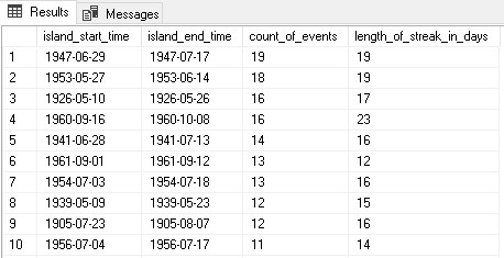
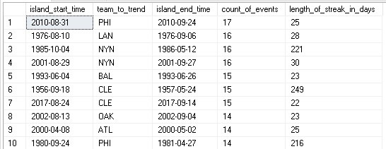
Note that all we have added here is a final select that joins together our CTEs on streak number (the island_number column). As a bonus, we can subtract island locations and find the difference between the start and end dates to determine how long a streak was, both in days and games. Ordering by streak length in games allows us to view the longest streaks first:

The results are straightforward and tell us the longest winning streaks of all time for a single team. Measuring losing streaks, tie streaks, or any other metric as a streak would only require changing the results that we define in the first CTE and then join on and filter in subsequent CTEs.

The syntax above seems lengthy, but now that it is defined, we can reuse it for all of our additional examples. We can customize and return a variety of more complicated insights without changing much about this code, making it a nice way to solve these analytic questions.

Using PARTITION BY to Calculate Streaks Across Multiple Entities

Analyzing winning streaks for a single team is useful, but what would be more interesting would be to look at a single team versus all other teams, or all teams versus all teams. This would provide an overall view of winning streaks, regardless of the opposition.

If we wanted to know the longest winning streaks by the Yankees versus other individual teams, we could accomplish that task by the use of PARTITION BY in all of our window functions. By partitioning by the opposing team, we can generate a list of winning streaks that are broken down into subsets for each team. With that single change, we can get a completely new set of results:

WITH GAME_LOG AS (
SELECT
    CASE WHEN (HomeScore > VisitingScore AND HomeTeamName = 'NYA')
            OR (VisitingScore > HomeScore AND VisitingTeamName = 'NYA')
            THEN 'W'
        WHEN (HomeScore > VisitingScore AND VisitingTeamName = 'NYA') 
            OR (VisitingScore > HomeScore AND HomeTeamName = 'NYA') 
            THEN 'L'
        WHEN VisitingScore = HomeScore THEN 'T'
    END AS result,
    LAG(CASE WHEN (HomeScore > VisitingScore AND HomeTeamName = 'NYA') 
                OR (VisitingScore > HomeScore 
                AND VisitingTeamName = 'NYA') 
                THEN 'W'
            WHEN (HomeScore > VisitingScore AND VisitingTeamName = 'NYA')
                OR (VisitingScore > HomeScore AND HomeTeamName = 'NYA')
                THEN 'L'
            WHEN VisitingScore = HomeScore THEN 'T' END) 
                OVER (PARTITION BY CASE WHEN VisitingTeamName = 'NYA'
                THEN HomeTeamName ELSE VisitingTeamName END
            ORDER BY GameLog.GameDate, GameLog.GameLogId) 
    AS previous_game_result,
    LEAD(CASE WHEN (HomeScore > VisitingScore AND HomeTeamName = 'NYA')
                OR (VisitingScore > HomeScore 
                AND VisitingTeamName = 'NYA') 
                THEN 'W'
            WHEN (HomeScore > VisitingScore 
                AND VisitingTeamName = 'NYA') 
                OR (VisitingScore > HomeScore AND HomeTeamName = 'NYA')
                THEN 'L'
            WHEN VisitingScore = HomeScore THEN 'T' END) 
                OVER (PARTITION BY CASE WHEN VisitingTeamName = 'NYA'
                THEN HomeTeamName ELSE VisitingTeamName END 
        ORDER BY GameLog.GameDate, GameLog.GameLogId) 
        AS next_game_result,
    ROW_NUMBER() 
        OVER (PARTITION BY CASE WHEN VisitingTeamName = 'NYA' 
                THEN HomeTeamName ELSE VisitingTeamName END 
                ORDER BY GameLog.GameDate, GameLog.GameLogId) 
        AS island_location,
    CASE WHEN VisitingTeamName = 'NYA' THEN HomeTeamName 
            ELSE VisitingTeamName END AS opposing_team, 
    GameLog.GameDate,
    GameLog.GameLogId
FROM dbo.GameLog
WHERE GameLog.GameType = 'REG'
    AND GameLog.HomeTeamName = 'NYA' 
    OR GameLog.VisitingTeamName = 'NYA'),
CTE_ISLAND_START AS (
SELECT
    ROW_NUMBER() OVER (PARTITION BY GAME_LOG.opposing_team 
        ORDER BY GAME_LOG.GameDate, GAME_LOG.GameLogId) 
        AS island_number,
    GAME_LOG.GameDate AS island_start_time,
    GAME_LOG.island_location AS island_start_location,
    GAME_LOG.opposing_team
FROM GAME_LOG
WHERE GAME_LOG.result = 'W'
    AND (GAME_LOG.previous_game_result <> 'W'
    OR GAME_LOG.previous_game_result IS NULL)),
CTE_ISLAND_END AS (
SELECT
    ROW_NUMBER() OVER (PARTITION BY GAME_LOG.opposing_team 
        ORDER BY GAME_LOG.GameDate, GAME_LOG.GameLogId) 
        AS island_number,
    GAME_LOG.GameDate AS island_end_time,
    GAME_LOG.island_location AS island_end_location,
    GAME_LOG.opposing_team
FROM GAME_LOG
WHERE GAME_LOG.result = 'W'
    AND (GAME_LOG.next_game_result <> 'W' 
    OR GAME_LOG.next_game_result IS NULL))
SELECT
    CTE_ISLAND_START.island_start_time,
    CTE_ISLAND_START.opposing_team,
    CTE_ISLAND_END.island_end_time,
    CTE_ISLAND_END.island_end_location - 
        CTE_ISLAND_START.island_start_location + 1 
        AS count_of_events,
    DATEDIFF(DAY, CTE_ISLAND_START.island_start_time, 
        CTE_ISLAND_END.island_end_time) + 1 
        AS length_of_streak_in_days
FROM CTE_ISLAND_START
INNER JOIN CTE_ISLAND_END
ON CTE_ISLAND_START.island_number = CTE_ISLAND_END.island_number
AND CTE_ISLAND_START.opposing_team = CTE_ISLAND_END.opposing_team
ORDER BY CTE_ISLAND_END.island_end_location 
    - CTE_ISLAND_START.island_start_location DESC;

Note that all window functions now include a PARTITION BY that operates on the opposing team. Window functions operate over a window, and here we are defining the window as a dataset per team. This means that we will have a window per team, rather than a single window for all teams.

For the GAME_LOG CTE, this calculation requires partitioning by a CASE statement that is similar to how we determined if a game was a win or loss. In the remaining CTEs, we can use the opposing_team column to more quickly generate these results (and with less code). Also, note the following:

The final SELECT is nearly identical to all previous demos.

CTE_ISLAND_START and CTE_ISLAND_END are identical to previous demos except in the use of PARTITION BY to further subdivide the dataset.

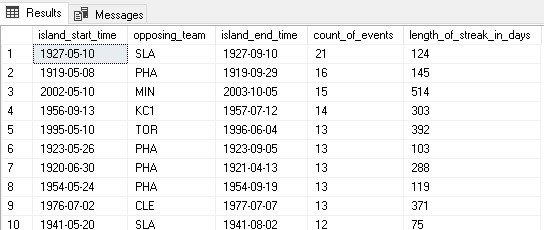
These similarities allow us to reuse the same syntax repeatedly with a high level of confidence in the results:

The results quickly tell us the longest winning streaks the Yankees have had versus all other teams in the regular season, with the St. Louis Browns being on the historical losing end of this dataset.

The dataset is interesting, but it begs the question: “How do we calculate winning streaks by all teams versus all teams?”. If we would like to see all winning streaks, regardless of team, then we will need to further customize our queries above as follows:

1. Include both home and visiting teams in all queries.

The GAME_LOG CTE needs to be adjusted with a UNION ALL to ensure that we get all games from the perspective of the home and away teams. In other words, we need to double the size of this CTE to ensure that we have a row per team per game.

1. This change will necessitate a separate CTE to appropriately order the dataset for further analysis.
2. Instead of partitioning by the opposing team, we need to partition by both the team to trend and the opposing team. This will generate a much larger set of windows to analyze.

The following is the final result of the changes above:

WITH GAME_LOG AS (
SELECT
    CASE WHEN HomeScore > VisitingScore THEN 'W'
         WHEN VisitingScore > HomeScore THEN 'L'
         WHEN HomeScore = VisitingScore THEN 'T'
    END AS result,
    VisitingTeamName AS opposing_team,
    HomeTeamName AS team_to_trend,
    GameLog.GameDate,
    GameLog.GameLogId
FROM dbo.GameLog
WHERE GameLog.GameType = 'REG'
UNION ALL
SELECT
    CASE WHEN VisitingScore > HomeScore THEN 'W'
         WHEN HomeScore > VisitingScore THEN 'L'
    END AS result,
    HomeTeamName AS opposing_team,
    VisitingTeamName AS team_to_trend,
    GameLog.GameDate,
    GameLog.GameLogId
FROM dbo.GameLog
WHERE GameLog.GameType = 'REG'
AND VisitingScore <> HomeScore),
GAME_LOG_ORDERED AS (
SELECT
    GAME_LOG.GameLogId,
    GAME_LOG.GameDate,
    GAME_LOG.team_to_trend,
    GAME_LOG.opposing_team,
    GAME_LOG.result,
    LAG(GAME_LOG.result) OVER (PARTITION BY team_to_trend, opposing_team 
            ORDER BY GAME_LOG.GameDate, GAME_LOG.GameLogId) 
                AS previous_game_result,
    LEAD(GAME_LOG.result) OVER (PARTITION BY team_to_trend, 
            opposing_team 
            ORDER BY GAME_LOG.GameDate, GAME_LOG.GameLogId) 
                AS next_game_result,
    ROW_NUMBER() OVER (PARTITION BY team_to_trend, opposing_team 
            ORDER BY GAME_LOG.GameDate, GAME_LOG.GameLogId) 
                AS island_location
FROM GAME_LOG),
CTE_ISLAND_START AS (
SELECT
    ROW_NUMBER() OVER (PARTITION BY GAME_LOG_ORDERED.team_to_trend, 
        GAME_LOG_ORDERED.opposing_team 
        ORDER BY GAME_LOG_ORDERED.GameDate, 
        GAME_LOG_ORDERED.GameLogId) 
        AS island_number,
    GAME_LOG_ORDERED.GameDate AS island_start_time,
    GAME_LOG_ORDERED.island_location AS island_start_location,
    GAME_LOG_ORDERED.opposing_team,
    GAME_LOG_ORDERED.team_to_trend
FROM GAME_LOG_ORDERED
WHERE GAME_LOG_ORDERED.result = 'W'
    AND (GAME_LOG_ORDERED.previous_game_result <> 'W' 
        OR GAME_LOG_ORDERED.previous_game_result IS NULL)),
CTE_ISLAND_END AS (
SELECT
    ROW_NUMBER() OVER (PARTITION BY GAME_LOG_ORDERED.team_to_trend, 
            GAME_LOG_ORDERED.opposing_team 
                ORDER BY GAME_LOG_ORDERED.GameDate, 
                GAME_LOG_ORDERED.GameLogId) 
                AS island_number,
    GAME_LOG_ORDERED.GameDate AS island_end_time,
    GAME_LOG_ORDERED.island_location AS island_end_location,
    GAME_LOG_ORDERED.opposing_team,
    GAME_LOG_ORDERED.team_to_trend
FROM GAME_LOG_ORDERED
WHERE GAME_LOG_ORDERED.result = 'W'
    AND (GAME_LOG_ORDERED.next_game_result <> 'W' 
        OR GAME_LOG_ORDERED.next_game_result IS NULL))
SELECT
    CTE_ISLAND_START.island_start_time,
    CTE_ISLAND_START.team_to_trend,
    CTE_ISLAND_START.opposing_team,
    CTE_ISLAND_END.island_end_time,
    CTE_ISLAND_END.island_end_location 
            - CTE_ISLAND_START.island_start_location + 1 
                AS count_of_events,
    DATEDIFF(DAY, CTE_ISLAND_START.island_start_time, 
            CTE_ISLAND_END.island_end_time) + 1 
                AS length_of_streak_in_days
FROM CTE_ISLAND_START
INNER JOIN CTE_ISLAND_END
ON CTE_ISLAND_START.island_number = CTE_ISLAND_END.island_number
AND CTE_ISLAND_START.opposing_team = CTE_ISLAND_END.opposing_team
AND CTE_ISLAND_START.team_to_trend = CTE_ISLAND_END.team_to_trend
ORDER BY CTE_ISLAND_END.island_end_location 
    - CTE_ISLAND_START.island_start_location DESC;

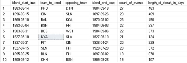
While the changes are readily apparent, the code overall is very similar to what we wrote earlier. Window functions operate over a window, and here we are defining the window as a dataset per each pair of teams. This means that we will have a window for every set of teams that have played each other. This is a far larger number of windows than earlier but is necessary to be able to calculate streaks in aggregate across all possible matchups. The results are as follows:

We can observe that the top winning streak for the Yankees is only number 6 on this list with the top 10 streaks ranging anywhere from 1883 to 1970. Streak lengths are often quite long as many spanned multiple seasons.

Longest Winning Streaks for Any Team

Another similar problem we may wish to solve is to determine the longest overall winning streaks for all teams in baseball. Earlier we calculated this metric for a single team, but there is value in being able to do so for all teams in a single query.

Fortunately, we have already done much of the work on this (and then some). To find the longest winning streaks for all teams in aggregate (not versus any specific team), all we need to do is remove the opposing team from all PARTITION BY clauses. The remaining TSQL remains nearly identical:

WITH GAME_LOG AS (
SELECT
    CASE WHEN HomeScore > VisitingScore THEN 'W'
         WHEN VisitingScore > HomeScore THEN 'L'
         WHEN HomeScore = VisitingScore THEN 'T'
    END AS result,
    VisitingTeamName AS opposing_team,
    HomeTeamName AS team_to_trend,
    GameLog.GameDate,
    GameLog.GameLogId
FROM dbo.GameLog
WHERE GameLog.GameType = 'REG'
UNION ALL
SELECT
    CASE WHEN VisitingScore > HomeScore THEN 'W'
            WHEN HomeScore > VisitingScore THEN 'L'
    END AS result,
    HomeTeamName AS opposing_team,
    VisitingTeamName AS team_to_trend,
    GameLog.GameDate,
    GameLog.GameLogId
FROM dbo.GameLog
WHERE GameLog.GameType = 'REG'
AND VisitingScore <> HomeScore),
GAME_LOG_ORDERED AS (
SELECT
    GAME_LOG.GameLogId,
    GAME_LOG.GameDate,
    GAME_LOG.team_to_trend,
    GAME_LOG.result,
    LAG(GAME_LOG.result) OVER (PARTITION BY team_to_trend 
            ORDER BY GAME_LOG.GameDate, GAME_LOG.GameLogId) 
                AS previous_game_result,
    LEAD(GAME_LOG.result) OVER (PARTITION BY team_to_trend 
            ORDER BY GAME_LOG.GameDate, GAME_LOG.GameLogId) 
                AS next_game_result,
    ROW_NUMBER() OVER (PARTITION BY team_to_trend 
            ORDER BY GAME_LOG.GameDate, GAME_LOG.GameLogId) 
                AS island_location
FROM GAME_LOG),
CTE_ISLAND_START AS (
SELECT
    ROW_NUMBER() OVER (PARTITION BY GAME_LOG_ORDERED.team_to_trend 
        ORDER BY GAME_LOG_ORDERED.GameDate, GAME_LOG_ORDERED.GameLogId) 
        AS island_number,
    GAME_LOG_ORDERED.GameDate AS island_start_time,
    GAME_LOG_ORDERED.island_location AS island_start_location,
    GAME_LOG_ORDERED.team_to_trend
FROM GAME_LOG_ORDERED
WHERE GAME_LOG_ORDERED.result = 'W'
    AND (GAME_LOG_ORDERED.previous_game_result <> 'W' 
        OR GAME_LOG_ORDERED.previous_game_result IS NULL)),
CTE_ISLAND_END AS (
SELECT
    ROW_NUMBER() OVER (PARTITION BY GAME_LOG_ORDERED.team_to_trend 
        ORDER BY GAME_LOG_ORDERED.GameDate, GAME_LOG_ORDERED.GameLogId) 
        AS island_number,
    GAME_LOG_ORDERED.GameDate AS island_end_time,
    GAME_LOG_ORDERED.island_location AS island_end_location,
    GAME_LOG_ORDERED.team_to_trend
FROM GAME_LOG_ORDERED
WHERE GAME_LOG_ORDERED.result = 'W'
    AND (GAME_LOG_ORDERED.next_game_result <> 'W' 
        OR GAME_LOG_ORDERED.next_game_result IS NULL))
SELECT
    CTE_ISLAND_START.island_start_time,
    CTE_ISLAND_START.team_to_trend,
    CTE_ISLAND_END.island_end_time,
    CTE_ISLAND_END.island_end_location - 
    CTE_ISLAND_START.island_start_location + 1 
        AS count_of_events,
    DATEDIFF(DAY, CTE_ISLAND_START.island_start_time, 
        CTE_ISLAND_END.island_end_time) + 1 
        AS length_of_streak_in_days
FROM CTE_ISLAND_START
INNER JOIN CTE_ISLAND_END
ON CTE_ISLAND_START.island_number = CTE_ISLAND_END.island_number
    AND CTE_ISLAND_START.team_to_trend = CTE_ISLAND_END.team_to_trend
ORDER BY CTE_ISLAND_END.island_end_location - 
CTE_ISLAND_START.island_start_location DESC;

Window functions operate over a window and here we are defining the window as a dataset per team. This means that we will have a single window for every team that has ever won a game. This contrasts our previous query, which generated far more windows to perform analysis over.

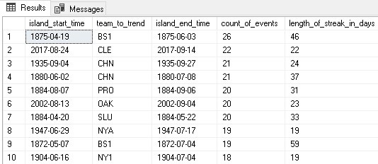
The results are as follows:

We can see that the longest winning streak of all time was accomplished by the Boston Red Stockings in 1875.

Note that the results do not include ties. Adjusting our work to include ties would require that we:

1. Change CTE_ISLAND_START and CTE_ISLAND_END to consider a streak start/end bounded by a loss, and not a loss or tie.
2. Adjust the count of events to exclude ties. This avoids reporting a streak that was more games won than were actually won.

Alternatively, we could count a tie as a win for record-keeping. This would simplify the T-SQL but report occasionally inaccurate data. For these metrics, adding a notes or has_ties column would better allow us to denote if a tie occurred.

The simplest approach would be to omit ties altogether and pretend they do not exist, like this:

WITH GAME_LOG AS (
SELECT
    CASE WHEN HomeScore > VisitingScore THEN 'W'
         ELSE 'L'
    END AS result,
    VisitingTeamName AS opposing_team,
    HomeTeamName AS team_to_trend,
    GameLog.GameDate,
    GameLog.GameLogId
FROM dbo.GameLog
WHERE GameLog.GameType = 'REG'
AND HomeScore <> VisitingScore
UNION ALL
SELECT
    CASE WHEN VisitingScore > HomeScore THEN 'W'
        ELSE 'L'
        END AS result,
    HomeTeamName AS opposing_team,
    VisitingTeamName AS team_to_trend,
    GameLog.GameDate,
    GameLog.GameLogId
FROM dbo.GameLog
WHERE GameLog.GameType = 'REG'
AND VisitingScore <> HomeScore),
GAME_LOG_ORDERED AS (
SELECT
    GAME_LOG.GameLogId,
    GAME_LOG.GameDate,
    GAME_LOG.team_to_trend,
    GAME_LOG.result,
    LAG(GAME_LOG.result) OVER (PARTITION BY team_to_trend 
        ORDER BY GAME_LOG.GameDate, GAME_LOG.GameLogId) 
        AS previous_game_result,
    LEAD(GAME_LOG.result) OVER (PARTITION BY team_to_trend 
        ORDER BY GAME_LOG.GameDate, GAME_LOG.GameLogId) 
        AS next_game_result,
    ROW_NUMBER() OVER (PARTITION BY team_to_trend 
        ORDER BY GAME_LOG.GameDate, GAME_LOG.GameLogId) 
        AS island_location
FROM GAME_LOG),
CTE_ISLAND_START AS (
SELECT
    ROW_NUMBER() OVER (PARTITION BY GAME_LOG_ORDERED.team_to_trend 
        ORDER BY GAME_LOG_ORDERED.GameDate, GAME_LOG_ORDERED.GameLogId)
        AS island_number,
    GAME_LOG_ORDERED.GameDate AS island_start_time,
    GAME_LOG_ORDERED.island_location AS island_start_location,
    GAME_LOG_ORDERED.team_to_trend
FROM GAME_LOG_ORDERED
WHERE GAME_LOG_ORDERED.result = 'W'
    AND (GAME_LOG_ORDERED.previous_game_result = 'L' 
    OR GAME_LOG_ORDERED.previous_game_result IS NULL)),
CTE_ISLAND_END AS (
SELECT
    ROW_NUMBER() OVER (PARTITION BY GAME_LOG_ORDERED.team_to_trend 
        ORDER BY GAME_LOG_ORDERED.GameDate, GAME_LOG_ORDERED.GameLogId)
        AS island_number,
    GAME_LOG_ORDERED.GameDate AS island_end_time,
    GAME_LOG_ORDERED.island_location AS island_end_location,
    GAME_LOG_ORDERED.team_to_trend
FROM GAME_LOG_ORDERED
WHERE GAME_LOG_ORDERED.result = 'W'
    AND (GAME_LOG_ORDERED.next_game_result = 'L' 
    OR GAME_LOG_ORDERED.next_game_result IS NULL))
SELECT
    CTE_ISLAND_START.island_start_time,
    CTE_ISLAND_START.team_to_trend,
    CTE_ISLAND_END.island_end_time,
    CTE_ISLAND_END.island_end_location 
        - CTE_ISLAND_START.island_start_location + 1 
        AS count_of_events,
    DATEDIFF(DAY, CTE_ISLAND_START.island_start_time, 
        CTE_ISLAND_END.island_end_time) + 1 
        AS length_of_streak_in_days
FROM CTE_ISLAND_START
INNER JOIN CTE_ISLAND_END
    ON CTE_ISLAND_START.island_number = CTE_ISLAND_END.island_number
    AND CTE_ISLAND_START.team_to_trend = CTE_ISLAND_END.team_to_trend
ORDER BY CTE_ISLAND_END.island_end_location 
    - CTE_ISLAND_START.island_start_location DESC;

This code explicitly filters out ties, so the end results will completely ignore them. We get no insight into whether a streak included ties but could easily join our result set back into the underlying data to gather that information, if it were important.

Filtering Results to Answer Obscure Questions

When observing any data analysis long enough, we are eventually surprised by obscure data requests or facts that might not come naturally to us. In sports, like in business, people are looking for new knowledge that can provide any statistical benefit. Does a player perform better at night? How about in the cold? Does being right or left-handed matter?

Statistics across these metrics sound mind-bogglingly complex but are incredibly easy to crunch using code we have already written. The key is to alter the filter of our primary dataset. The remainder of the gaps/islands analysis can be left as-is and will perform exactly as we want.

For example, imagine we wanted to track winning streaks for all teams at night. The T-SQL to make this happen is as follows:

WITH GAME_LOG AS (
SELECT
    CASE WHEN HomeScore > VisitingScore THEN 'W'
        WHEN VisitingScore > HomeScore THEN 'L'
        WHEN HomeScore = VisitingScore THEN 'T'
    END AS result,
    VisitingTeamName AS opposing_team,
    HomeTeamName AS team_to_trend,
    GameLog.GameDate,
    GameLog.GameLogId
FROM dbo.GameLog
WHERE GameLog.GameType = 'REG'
AND GameLog.DayorNight = 'N'
AND GameLog.DayorNight IS NOT NULL
UNION ALL
SELECT
    CASE WHEN VisitingScore > HomeScore THEN 'W'
            WHEN HomeScore > VisitingScore THEN 'L'
    END AS result,
    HomeTeamName AS opposing_team,
    VisitingTeamName AS team_to_trend,
    GameLog.GameDate,
    GameLog.GameLogId
FROM dbo.GameLog
WHERE GameLog.GameType = 'REG'
AND GameLog.DayorNight = 'N'
AND GameLog.DayorNight IS NOT NULL
AND VisitingScore <> HomeScore),
GAME_LOG_ORDERED AS (
SELECT
    GAME_LOG.GameLogId,
    GAME_LOG.GameDate,
    GAME_LOG.team_to_trend,
    GAME_LOG.result,
    LAG(GAME_LOG.result) OVER (PARTITION BY team_to_trend 
        ORDER BY GAME_LOG.GameDate, GAME_LOG.GameLogId) 
        AS previous_game_result,
    LEAD(GAME_LOG.result) OVER (PARTITION BY team_to_trend 
        ORDER BY GAME_LOG.GameDate, GAME_LOG.GameLogId) 
        AS next_game_result,
    ROW_NUMBER() OVER (PARTITION BY team_to_trend 
        ORDER BY GAME_LOG.GameDate, 
        GAME_LOG.GameLogId) AS island_location
FROM GAME_LOG),
CTE_ISLAND_START AS (
SELECT
    ROW_NUMBER() OVER (PARTITION BY GAME_LOG_ORDERED.team_to_trend 
        ORDER BY GAME_LOG_ORDERED.GameDate, GAME_LOG_ORDERED.GameLogId) 
        AS island_number,
    GAME_LOG_ORDERED.GameDate AS island_start_time,
    GAME_LOG_ORDERED.island_location AS island_start_location,
    GAME_LOG_ORDERED.team_to_trend
FROM GAME_LOG_ORDERED
WHERE GAME_LOG_ORDERED.result = 'W'
    AND (GAME_LOG_ORDERED.previous_game_result <> 'W' 
    OR GAME_LOG_ORDERED.previous_game_result IS NULL)),
CTE_ISLAND_END AS (
SELECT
    ROW_NUMBER() OVER (PARTITION BY GAME_LOG_ORDERED.team_to_trend 
        ORDER BY GAME_LOG_ORDERED.GameDate, GAME_LOG_ORDERED.GameLogId) 
        AS island_number,
    GAME_LOG_ORDERED.GameDate AS island_end_time,
    GAME_LOG_ORDERED.island_location AS island_end_location,
    GAME_LOG_ORDERED.team_to_trend
FROM GAME_LOG_ORDERED
WHERE GAME_LOG_ORDERED.result = 'W'
    AND (GAME_LOG_ORDERED.next_game_result <> 'W' 
    OR GAME_LOG_ORDERED.next_game_result IS NULL))
SELECT
    CTE_ISLAND_START.island_start_time,
    CTE_ISLAND_START.team_to_trend,
    CTE_ISLAND_END.island_end_time,
    CTE_ISLAND_END.island_end_location 
        - CTE_ISLAND_START.island_start_location + 1 
        AS count_of_events,
    DATEDIFF(DAY, CTE_ISLAND_START.island_start_time, 
        CTE_ISLAND_END.island_end_time) + 1 AS length_of_streak_in_days
FROM CTE_ISLAND_START
INNER JOIN CTE_ISLAND_END
ON CTE_ISLAND_START.island_number = CTE_ISLAND_END.island_number
    AND CTE_ISLAND_START.team_to_trend = CTE_ISLAND_END.team_to_trend
ORDER BY CTE_ISLAND_END.island_end_location 
    - CTE_ISLAND_START.island_start_location DESC;

The only change is that we added a filter to each part of the UNION dataset to filter out all games that are not night games. We check for NULL as some older games have no record of time of day. The results are as follows:

The results provide some obscure, but interesting data. Oftentimes, scenarios like these will seem nonsensical until a real-world scenario arises where they make perfect sense. For many statistical analyses, being able to improve predictions even by a small percentage can have a profound impact. For job functions such as sales or marketing, timing questions arise often and knowing the optimal ways in which to engage people can be the difference between success and failure.

Conclusion

The TSQL introduced in this article was not for the faint of heart. Breaking it into smaller pieces and viewing each chunk as a logical step towards getting our result set helped make it easier to read and understand. To summarize, the general process used in every islands/streaks analysis:

1. Create a dataset with a definitive win/loss definition.
2. Order the dataset so that each event can be numbered.
3. Generate a list of island starting points
4. Generate a list of island ending points
5. Join the starting and ending points together and return results.

Once this syntax is established, every query will be similar to the rest of the queries we write. Copying, pasting, and modifying this TSQL to create new filters, partitions, or metrics is recommended as a far faster and reliable alternative than rewriting this code repeatedly.

Using this style of analysis, we can crunch vast amounts of data into meaningful groups that can measure success and report on how events relate to other nearby events. While other tools such as Python or R can be used to crunch this data in a similar fashion, being closer to the data allows for easier customization and more reliable control over performance.

 

The post Efficient Solutions to Gaps and Islands Challenges appeared first on Simple Talk.

from Simple Talk https://ift.tt/30ExEAe
via

Speaking at Nashville SQL Saturday this weekend

Boy does time fly, and it is already mid January. The holidays flew by, and now the Christmas tree and (most of) the Christmas décor has been boxed up in the attic (yeah, there is a Santa on a shelf staring at me that he needs to be put up!). The college bowl games are over, rendering all college teams a blissful 0-0 record again, and in the SQL Server community area, one of the very first events is upon us: SQL Saturday Nashville.

This year, I am speaking in the first slot at 8:30, talking out that favorite topic of mine: The fundamentals Relational Database Design. Even if you are not going to be building databases and are just writing code to use them, understanding why the data architect gets really grumpy when a database has 2 tables with 1000 columns each (even though it “gets the job done, I suppose”) will at least let you know the issues you might run into with less than optimal designs.

I have been doing a variation of this presentation for 20 years, and while the reasons to build a relational database a certain way haven’t changed, a lot has changed as to why it is so important to at least understand the basics. The amount of data being stored, even for simple transactions, has skyrocketed over the years, and businesses are looking for more information from their data than just knowing that a product was shipped, and that we got paid for it. The big question people want to know is “how do we get them to do it again with the least amount of effort?” To do that calculation, the better the data, the easier the calculation.

The abstract for the presentation is:

Data should be easy to work with in SQL Server if the database has been organized as close as possible to the standards of normalization that have been proven for many years, but are often thought of as old-fashioned. Many common T-SQL programming “difficulties” are the result of struggling against these standards and can be avoided by understanding the requirements, applying normalization, as well as a healthy dose of simple common sense. In this session I will give an overview of how to design a relational database, allowing you to work with the data structures instead of against them. This will let you use SQL naturally, enabling the query engine internals to optimize your output needs without you needing to spend a lot of time thinking about it. This will mean less time trying to figure out why SUBSTRING(column,3,1) = ‘A’ is killing your performance, and more time for solving the next customer problem.

Of course, all of this is a very tall order for an hour, and when I did this as a webinar for SentryOne with the fabulous Kevin Kline as my color commentator, it took about 2 hours, over two sessions (the second one is here). So come to see it live, or check it out on your own pace because you had rather go see Monica Rathbun talk about performance. Hey, if you build tables and don’t care about the right way to design a relational database is probably a good idea anyhow. Though I do expect one of her items might be (don’t do a crappy job designing in the first place!)

Hope to see you there!

The post Speaking at Nashville SQL Saturday this weekend appeared first on Simple Talk.

from Simple Talk https://ift.tt/2QXzVDx
via

Capturing a Mind

When the Netflix series Black Mirror began in 2011, I watched a few episodes. Recently, I “binge-watched” more to catch up. If you’re not familiar with the series, each episode is about technology, and how people must deal with it when it goes awry. For the most part, the technology featured in the series doesn’t exist…yet.

One episode from 2016, Nosedive, is almost too close for comfort. As people interact, they give each other ratings much like giving an Uber driver or passenger a rating today. A person’s rating determines how others in society treat them and the opportunities that they have. Once a rating drops too low, it’s almost impossible to climb back up. The characters accept that whole situation is normal, and it is similar to how we have accepted the intrusion to our privacy from social media like Facebook today.

Since I was watching several episodes in one weekend, I noticed a theme: the ability to copy a person’s mind into a “cookie” that can interact with other people. In each case, the copy thought they were the real thing. In one episode, a scientist took a cookie from a convict as he was executed. The scientist then placed the cookie in a museum where tourists could execute the “man” over and over without eliminating him. This was terrible torture as he could feel the pain and agony each time.

In another case, a husband had the cookie of his comatose wife implanted into him. This allowed her to see and feel everything he experienced which was great for interacting with their son. You can probably imagine the problems that came up as the husband tried to live his life with this implant, and the husband eventually agreed to place her into a toy that their son soon abandoned. By the way, she ended up in the same museum as the convict.

Police used a cookie to extract a confession in one episode, and a software developer punished his co-workers by putting copies of them into a video game of his favourite TV show.

In each case, the real humans didn’t care much about the rights or experiences of the cookies, and the ethical and legal questions come up quite often. Is it legal to terminate a copy of a mind? Is it ethical to put a copy on pause or give it nothing to do for several months?

Even though this series is science fiction, I wonder how far away we are from achieving some of the technology featured. Capturing an entire mind does seem far off, but many things we accept today were science fiction not too long ago.

 

The post Capturing a Mind appeared first on Simple Talk.

from Simple Talk https://ift.tt/2ZZtdQm
via

But the Database Worked in Development! Preventing Broken Constraints

You’re working in development, releasing a new version of the application. You’ve temporarily disabled constraints in the new version of the database, you’ve imported the current data, your hand is poised to enable constraints. Is it going to spring errors at you? What if it does?

Or, what if you synchronize a source with a target by changing the metadata, only to find that the process has an error saying a constraint, index or foreign key can’t be created?

How could this happen? What has happened in both cases is that the data does not comply with the constraints. Maybe you’ve added or altered some constraints, and you have tested them on a different version of the data, changing this data slightly to satisfy the new constraints but without providing your changes as a data migration script. Perhaps you’ve only tested the new or altered constraints using an artificial data set, with no troublesome duplicates or broken references? Possibly, you are working in development and staging is done by a different team. Deployment and release are often, from necessity, done by a different team to development. You release the new database version to staging, which perhaps is managed by a different team, and when they try to update the existing database to the new build, the build breaks.

Often, at this point, one or other of the teams will need to repeatedly try releasing while fixing all the bad data, one error message at a time. This isn’t going to help team bonding; you need a better way of dealing with these problems.

In this series of articles, I’ll provide a more reliable way to be able to tease out all the duplicates, the broken foreign key references or all the values that will cause CHECK constraint errors, before you run a deployment. It will not only report where the errors would occur, but which data in which tables would cause which constraints to fail.

Dealing with Data that Breaks the Build

Sometimes a database build breaks only when you try to release it to staging or, worse, to production. Up to that point everything is sweetness and light. Then you either synchronise or try to load the data. What has happened? Well, it could be that in the new version of the databases, you’ve added DEFAULT constraints, FOREIGN KEYs or unique indexes, as you should, or modified existing keys and constraints to enforce referential integrity, and do a better job at preventing ‘bad data’ from creeping into the database.

If you are very fortunate, you will have access to the real data, so you can enable constraints one at a time and, when one causes an error, fix the data that is recorded in the error, and develop the scripts to heal the data in a pre-deployment script in order to remove the duplicates and bad data and fix the broken FOREIGN KEY references that initially inspired you to do the work.

There’s nothing wrong with that sort of data migration script, of course, although it requires a lot of careful work, gathering up all the de-duplicating statements, making them idempotent, testing them, and then using them in a pre-deployment script for a release. Even after all this, new data may have been inserted into Production, since you took the backup for testing, which might still break the build. If you are importing the existing data into a new build, then you would disable all constraints, import the data, heal it in-situ with the data-migration script and then finally enable constraints.

What, though, if you can’t access the production data, for several good reasons? In this case, you’re most likely testing with an artificially generated set of data for testing or a masked copy of the production data. However, unless you are one of the wild men of IT, it isn’t the actual production data, and so doesn’t have all the real data’s failings. Now, either the Ops team will need to try to fix all the duplicates and bad data, until the build succeeds, or they will pass the baton back to you.

Unless you enjoy buying all the drinks on the Friday afternoon DevOps team meeting, you must never deliberately break the database build or release. What you need to do is to provide a way that the Ops people can check the data of the target database beforehand to make sure it will pass all the checks done by constraints and unique indexes, and that all the FOREIGN KEY references are in place. If it doesn’t, and this is the key difference, they will need a report of what data failed the new constraints, so that you can provide scripts to allow DevOps people to fix the data.

When you know what is failing, you can create the deduplication, broken FOREIGN KEY reference or data-sanitizing scripts. Then you re-test until you get a clean bill of health. Although I can’t really help with the actual de-duplication, I can, in this article, help you to generate the list of the constraints that will fail and why.

Duplicates

Duplicates are like rats: they get in unless you take active steps to stop them. Data just seems to want to reproduce itself. The grey-muzzled database developer will take elaborate steps to check for duplicates everywhere by using unique constraints, whilst the cub developers snigger amongst themselves at how impossible it would be for a duplicate to get in there anyway. The blighters always insinuate themselves wherever there are no checks against them. Duplicates, I mean, rather than cub developers. This means that every database revision seems to have more uniqueness checks, inspired by the labour of teasing duplicates out and stamping on them. If the production data has duplicates, this must be fixed before you can release new unique constraints successfully to that target database.

Constraints and Bad Data

However often I go on about CHECK constraints, there will always be a developer who will leave them out or mutter in a dignified manner about how all checks need to be done only at the application level. This attitude soon gets divine retribution. Bad data springs up like a rotting fungus over your database unless you add CHECK constraints to all your tables. This is fine but then how do you prevent the excellent and estimable habit of adding them to then interfere with a release? The constraints will stop the build if they meet bad data: it is what they are trained to do. If you don’t like that, then you must fix the bad data first.

Unreferenced Foreign Keys

These are less frequent, but I’ve seen them. What happens here is that you import your data, enable constraints, and you get a message about a foreign key reference. This happens if, for example, the name of a country that is referenced in an address list or currency table is missing. Getting data right in a referenced table can be like picking up lots of tadpoles and putting them in a jar. Unless you know what failed, this can be very tricky to fix.

Checking the CHECK Constraints: First Principles

We’ll show how to do a check. The whole point of this type of test is that it must report the breakages in enough detail that you can smilingly pass to the Ops Guy a script that will heal it.

Let’s do the very simplest check: a check of constraints. We’ll do this by assembling a batch as a string. This batch will execute every constraint in the database, on the table to which it belongs, and tot up the grand total of rows that failed a constraint.

DECLARE @AllTheFailures INT; --tally of all the 
   --failures in the constraints
DECLARE @CheckAllYourConstraints NVARCHAR(MAX) = 
   'Select @RowsFailed =0;
';
SELECT @CheckAllYourConstraints = 
   @CheckAllYourConstraints --accumulate each query
  + N'
    Select @RowsFailed=@RowsFailed+count(*) from ' --the table spec
  + QuoteName(Object_Schema_Name(CC.parent_object_id)) + N'.'
  + QuoteName(Object_Name(CC.parent_object_id)) + N' WHERE NOT ' 
  + definition
  FROM sys.check_constraints AS CC
  WHERE is_ms_shipped = 0;
--Now we have a list of select queries that will accumulate 
--the total number of rows that fail the condition
EXECUTE sp_executesql @CheckAllYourConstraints, 
  N'@RowsFailed int output',
  @RowsFailed = @AllTheFailures OUTPUT;
SELECT @AllTheFailures;

We run this in our test copy of AdventureWorks2016. It returns no rows, because all the constraints are enabled and so the rows are already well-policed by those constraints if they are in a ‘trusted’ state.

The batch that was executed was this:

Select @RowsFailed =0;
Select @RowsFailed=@RowsFailed+count(*) from [Person].[Person] 
WHERE NOT ([EmailPromotion]>=(0) AND [EmailPromotion]<=(2))
Select @RowsFailed=@RowsFailed+count(*) from [Sales].[SalesTaxRate] 
WHERE NOT ([TaxType]>=(1) AND [TaxType]<=(3))
Select @RowsFailed=@RowsFailed+count(*) from [Sales].[SalesTerritory] 
WHERE NOT ([SalesYTD]>=(0.00))
Select @RowsFailed=@RowsFailed+count(*) from [Sales].[SalesTerritory] 
WHERE NOT ([SalesLastYear]>=(0.00))
Select @RowsFailed=@RowsFailed+count(*) from [Production].[Product] 
WHERE NOT ([SafetyStockLevel]>(0))
Select @RowsFailed=@RowsFailed+count(*) from [Sales].[SalesTerritory] 
WHERE NOT ([CostYTD]>=(0.00))
…and so on.

Now we’ll mangle our copy of AdventureWorks2016. Don’t worry, since it is a clone maintained by SQL Clone, I can do what I like and refresh it when I want it back to its pristine state. We’ll disable a constraint and alter the data so that when I try to reenable it, it will fail. Dave the Dev of AdventureWorks has decided that the MaritalStatus code in the employee table needs more options than M for married or S for single. What about P for Partner? He disables the CHECK constraint, CK_Employee_MaritalStatus.

ALTER TABLE humanResources.employee 
NOCHECK CONSTRAINT CK_Employee_MaritalStatus

Then he makes the necessary changes.

UPDATE humanresources.employee SET maritalStatus='P' 
WHERE BusinessEntityID=1  
UPDATE humanresources.employee SET maritalStatus='P' 
WHERE BusinessEntityID=7  
UPDATE humanresources.employee SET maritalStatus='P' 
WHERE BusinessEntityID=11 
UPDATE humanresources.employee SET maritalStatus='P' 
WHERE BusinessEntityID= 14 
UPDATE humanresources.employee SET maritalStatus='P' 
WHERE BusinessEntityID=17 
UPDATE humanresources.employee SET maritalStatus='P' 
WHERE BusinessEntityID=18 
UPDATE humanresources.employee SET maritalStatus='P' 
WHERE BusinessEntityID= 19

Developer Dave is just getting ready to change the constraint and enable it when he is called into an important team discussion, and he forgets.

Now we’ll rerun the code to monitor constraints. It will tell you that seven rows failed. It doesn’t tell you which rows in which table, and for which constraint. It is nice to have, but we’d want even more for the code to be useful.

If you want to play along and you don’t have SQL Clone, that is fine. We can replace the code this way once you’re done with testing.

UPDATE humanresources.employee SET maritalStatus='S' 
WHERE BusinessEntityID=1  
UPDATE humanresources.employee SET maritalStatus='M' 
WHERE BusinessEntityID=7  
UPDATE humanresources.employee SET maritalStatus='S' 
WHERE BusinessEntityID=11 
UPDATE humanresources.employee SET maritalStatus='S' 
WHERE BusinessEntityID= 14 
UPDATE humanresources.employee SET maritalStatus='S' 
WHERE BusinessEntityID=17 
UPDATE humanresources.employee SET maritalStatus='S' 
WHERE BusinessEntityID=18 
UPDATE humanresources.employee SET maritalStatus='S' 
WHERE BusinessEntityID= 19
ALTER TABLE humanResources.employee WITH CHECK 
CHECK CONSTRAINT CK_Employee_MaritalStatus

We can also alter what is in a constraint in order to simulate a problem

ALTER TABLE Production.Product DROP CONSTRAINT CK_Product_ProductLine;
GO
ALTER TABLE Production.Product WITH NOCHECK
ADD CONSTRAINT CK_Product_ProductLine
  --CHECK (upper([ProductLine])='R' OR upper([ProductLine])='M' 
  --  OR upper([ProductLine])='T' OR upper([ProductLine])='S' 
  --  OR [ProductLine] IS NULL); 
  CHECK (Upper(ProductLine) = 'A'
      OR Upper(ProductLine) = 'B'
      OR Upper(ProductLine) = 'C'
      OR Upper(ProductLine) = 'D'
      OR ProductLine IS NULL
        );

This constraint is set as disabled in this code; otherwise it wouldn’t execute without an error since the existing data fails the check.

You can run the test and then check that the code has picked up the problem. Then when you are finished, you can revert the change or, in my case, revert the clone.

ALTER TABLE Production.Product DROP CONSTRAINT CK_Product_ProductLine;
GO
ALTER TABLE Production.Product WITH NOCHECK
ADD CONSTRAINT CK_Product_ProductLine
  CHECK (upper([ProductLine])='R' OR upper([ProductLine])='M' 
  OR upper([ProductLine])='T' OR upper([ProductLine])='S' 
  OR [ProductLine] IS NULL);

Which Rows Violated which Constraints?

Now we decide what we really want. I can be sure that I want a copy of all the metadata about CHECK constraints in source control with each build, generated after the first build, so I can then test all the subsequent data sets in the deployment chain to make sure they are free from ‘breaking data’.

To store this information means a JSON document because it is text-based, and this can be more versatile. We are likely to need to test data held in a different version of the database, so we abandon the idea of using the metadata directly. I also like to know more about the data that was selected as failing the test. I would like the name of the table and the name of the constraint. I need where possible, to see a good sample of the data though this isn’t possible or necessary with CHECK constraints. We need to get more serious about the tests, even if we lose some of the elegance of the code. One other thing is necessary once we decide to make it possible to run this on other versions of the database: In the case of unique indexes and FOREIGN KEY constraints, we need to check whether all the columns and tables involved are there under the same name. With CHECK constraints, all we can realistically do is to check for the table’s existence.

Here is an example of the report we get:

It is easy to see what is wrong in the data. That MaritalStatus column will need to be either ‘M‘ or ‘S‘ until Developer Dave fixes the constraint.

My apologies that this sort of convenience makes for more code.

DROP PROCEDURE IF EXISTS #ListAllCheckConstraints;
GO
CREATE PROCEDURE #ListAllCheckConstraints
  /**
Summary: >
  This creates a JSON list of all the check constraints in the database. 
  their name, table and definition
Author: Phil Factor
Date: 12/12/2019
Example:
   - DECLARE @OurListAllCheckConstraints  NVARCHAR(MAX)
     EXECUTE #ListAllCheckConstraints 
           @TheJsonList=@OurListAllCheckConstraints OUTPUT
     SELECT @OurListAllCheckConstraints AS theCheckConstraints
   - DECLARE @OurCheckConstraints  NVARCHAR(MAX)
     EXECUTE #ListAllCheckConstraints 
           @TheJsonList=@OurCheckConstraints OUTPUT
     SELECT Constraintname, TheTable, [definition]
      FROM OPENJSON(@OurCheckConstraints)  WITH
      (Constraintname sysname '$.constraintname',
           TheTable sysname '$.thetable', 
      [Definition] nvarchar(4000) '$.definition' ); 
Returns: >
  the JSON as an output variable
**/
  @TheJSONList NVARCHAR(MAX) OUTPUT
AS
SELECT @TheJSONList =
  (
  SELECT QuoteName(CC.name) AS constraintname,
    QuoteName(Object_Schema_Name(CC.parent_object_id)) + '.'
    + QuoteName(Object_Name(CC.parent_object_id)) AS thetable, 
    definition
    FROM sys.check_constraints AS CC
    WHERE is_ms_shipped = 0
  FOR JSON AUTO
  );
GO
DROP PROCEDURE IF EXISTS #TestAllCheckConstraints;
GO
CREATE PROCEDURE #TestAllCheckConstraints
  /**
Summary: >
  This tests the current database against its check constraints. 
  and reports any data that would fail a check were it enabled
Author: Phil Factor
Date: 15/12/2019
Example:
   - DECLARE @OurFailedConstraints  NVARCHAR(MAX)
     EXECUTE #TestAllCheckConstraints 
          @TheResult=@OurFailedConstraints OUTPUT
     SELECT @OurFailedConstraints AS theFailedCheckConstraints
  Returns: >
  the JSON as an output variable
**/
@JsonConstraintList NVARCHAR(MAX)=null,--you can either provide 
   --a json document or you can go and get the current
@TheResult NVARCHAR(MAX) OUTPUT --the JSON document that gives 
   --the test result.
as
IF @JsonConstraintList IS NULL
  EXECUTE #ListAllCheckConstraints 
      @TheJSONList = @JsonConstraintList OUTPUT;
DECLARE @Errors TABLE (Description NVARCHAR(MAX));--to temporarily 
      --hold errors
DECLARE @Breakers TABLE (TheObject NVARCHAR(MAX));--the rows that 
      --would fail
DECLARE @TheConstraints TABLE --the list of check constraints 
      --in the database
  (
  TheOrder INT IDENTITY PRIMARY KEY, --needed to iterate 
     --through the table
  ConstraintName sysname, --the number of columns used in the index
  TheTable sysname, --the quoted name of the table wqith the schema
  Definition NVARCHAR(4000) --the actual code of the constraint
  );
--we put the constraint data we need into a table variable
INSERT INTO @TheConstraints (ConstraintName, TheTable, Definition)
  SELECT Constraintname, TheTable, Definition
    FROM OpenJson(@JsonConstraintList)
    WITH --get the relational table from the JSON
      (
      Constraintname sysname '$.constraintname', 
       TheTable sysname '$.thetable',
      Definition NVARCHAR(4000) '$.definition' --the mapping
      );
DECLARE @iiMax INT = @@RowCount;
--to do the actual check
DECLARE @CheckConstraintExecString NVARCHAR(4000);
--make sure the table is there
DECLARE @TestForTableExistenceString NVARCHAR(4000);
--to get a sample of broken rows
DECLARE @GetBreakerSampleExecString NVARCHAR(4000);
--temporarily hold the current constraint name
DECLARE @ConstraintName sysname;
--temporarily hold the current constraint's table
DECLARE @ConstraintTable sysname;
--temporarily hold the constraint code
DECLARE @ConstraintExpression NVARCHAR(4000);
--the number of rows that fail the current constraint
DECLARE @AllRowsFailed INT; 
--a sample of failed rows
DECLARE @SampleOfFailedRows NVARCHAR(MAX);
--Did the table exist in the current database
DECLARE @ThereWasATable INT;
DECLARE @ii INT = 1;--iteration variables
WHILE (@ii <= @iiMax)
  --------------------start of the loop------------------
  BEGIN --create the expressions we need to execute 
        --dynamically for each constraint
    SELECT @CheckConstraintExecString = --expression that checks 
                                        --the constraint
      N'SELECT @RowsFailed=Count(*) FROM ' + TheTable + N' WHERE NOT '
      + Definition, @ConstraintName = ConstraintName,
      @ConstraintTable = TheTable,
      @GetBreakerSampleExecString = --expression that gets 
                                    --sample of failed rows
        N'SELECT @JSONBreakerData= (Select top 3 * FROM ' + TheTable
        + N' WHERE NOT ' + Definition + N'FOR JSON AUTO)',
      @ConstraintName = ConstraintName, @ConstraintTable = TheTable,
      @ConstraintExpression=[definition],
      @TestForTableExistenceString = --expression that checks 
                                     --for the table
        N'SELECT @TableThere=case when Object_id(''' + TheTable
        + N''') is null then 0 else 1 end'
      FROM @TheConstraints
      WHERE TheOrder = @ii;
      --check that the table is there 
    EXECUTE sp_executesql @TestForTableExistenceString,
      N'@TableThere int output', @TableThere = @ThereWasATable OUTPUT;
    IF @ThereWasATable = 1
      BEGIN --it is a bit safer to check the constraint
        EXECUTE sp_executesql @CheckConstraintExecString,
          N'@RowsFailed int output', @RowsFailed = @AllRowsFailed OUTPUT;
        IF @AllRowsFailed > 0 --Ooh, at least one failed constraint
          BEGIN--so we get a sample of the bad data in JSON
            EXECUTE sp_executesql @GetBreakerSampleExecString,
              N'@JSONBreakerData nvarchar(max) output',
              @JSONBreakerData = @SampleOfFailedRows OUTPUT;
            INSERT INTO @Breakers (TheObject)
              SELECT--and save the sample of bad rows along with 
                    --information about the constraint
                (
                SELECT 
                  Convert(VARCHAR(10), @AllRowsFailed) AS RowsFailed,
                  @ConstraintName AS ConstraintName,
                  @ConstraintTable AS ConstraintTable,
                  @ConstraintExpression AS Expression,
                  Json_Query(@SampleOfFailedRows) AS BadDataSample
                FOR JSON PATH, WITHOUT_ARRAY_WRAPPER
                );
          END;
      END;
    ELSE INSERT INTO @Errors (Description) 
         SELECT 'We Couldn''t find the table '
+ @ConstraintTable;
    SELECT @ii = @ii + 1; -- and iterate to the next row
  END;
 SELECT @TheResult= -- so we construct the JSON report.
  (SELECT
    (SELECT Json_Query(TheObject) AS BadData 
     FROM @Breakers FOR JSON AUTO) AS FailedChecks,
  (SELECT Description FROM @Errors FOR JSON AUTO) AS errors
FOR JSON PATH);
go

The first job the code does, using the temporary procedure #ListAllCheckConstraints is to create, from the development database a JSON-based list of all the check constraints that you can then use for the test. The obvious place to get this information from is the new build of the database. You don’t need any database data at this point as we’re just interested in the metadata. We just want to know what to check once you’ve imported the data and before you enable constraints.

With this data, stored as a JSON document to make it portable, we can then test the data within the target database this is done by #TestAllCheckConstraints

DECLARE @OurFailedConstraints  NVARCHAR(MAX)
     EXECUTE #TestAllCheckConstraints 
        @TheResult=@OurFailedConstraints OUTPUT
     SELECT @OurFailedConstraints AS theFailedCheckConstraints

You can then run all the tests on the target database automatically, using the data in this JSON document. If the table no longer exists, it will report the fact and avoid an error by bypassing the constraint check. Ideally, the check should really be in the pre-deployment script because you may decide that you want to prevent the build from going ahead if there is bad data in a column.

Here is an error where I’ve duplicated a row. This indicates that you will not be able to enable the index AK_SalesTaxRate_StateProvinceID_TaxType or AK_SalesTaxRate_rowguid without getting an error. It is telling you what duplicates will cause the error.

[{
    "duplicatelist": [{
        "duplicated": {
            "indexName": "AK_SalesTaxRate_StateProvinceID_TaxType",
            "tablename": "[Sales].[SalesTaxRate]",
            "columnlist": "[StateProvinceID],[TaxType]",
            "duplicates": [{
                "duplicatecount": 2,
                "StateProvinceID": 1,
                "TaxType": 1
            }]
        }
    }, {
        "duplicated": {
            "indexName": "AK_SalesTaxRate_rowguid",
            "tablename": "[Sales].[SalesTaxRate]",
            "columnlist": "[rowguid]",
            "duplicates": [{
                "duplicatecount": 2,
                "rowguid": "683DE5DD-521A-47D4-A573-06A3CDB1BC5D"
            }]
        }
    }]
}]

You will, however, be relieved that there is no ‘errors’ array in this document. Yes, it is easy to test. Why would you be relieved? This is because, if there were errors, the routine would be telling you that for one or more of the tests, either the table or one of the columns is missing. It does this check first, and if it knows that the duplicate check couldn’t even run, it doesn’t do it. You have a minor but tedious problem if you’ve changed the table columns used in these indexes as part of the release. This is because you’ll need to amend the list to allow an automated test, but this will be a relatively minor task. The script to make changes requires judgement and is not easily automated, but an existence-check for the columns is there and the information yielded should make a repair easy.

Another concern is that you may want to only test for certain constraints. As tables get much larger, it just takes too long. You only want to do them where you are putting in a new or changed constraint. Here, the answer is simple: you store the JSON document in source control and generate a new JSON document that lists just the new or altered constraints to be tested.

Summary

One aspect of DevOps teamwork involves a sort of remote running of test software. You as a developer devise the test, it is run by someone else under circumstances you can’t directly control, and you get back a report that gives you enough information to fix any problems that come up. It is curiously like the old Sybase technique of sending queries via email to be run, but without the scary surface-area exposure.

This type of test should avoid throwing errors and should collect all the information you need to script out a solution. It should not add work for the person who runs the script.

In the next article, we’ll add the routines for foreign key references and unique constraints. Armed with these, we can tie it all together to show how it fits in with a sophisticated deployment system such as SCA.

 

The post But the Database Worked in Development! Preventing Broken Constraints appeared first on Simple Talk.

from Simple Talk https://ift.tt/39T9l5I
via

Comments and More in PowerShell

As with any programming language, PowerShell supports comments. In fact, it will support two styles of comments. However, as you will see later in this article, PowerShell can use comments in a couple of interesting and unexpected ways that can be quite powerful.

Using Comments

The most common style of comment you will see is a line preceded with a # symbol. (I leave it to you to decide if you want to call that a hashtag, a pound symbol, or even a good old octothorpe!)

As an example, you might have a comment block at the start of your program with details about it:

#This is an example of single-line comments
#
#Author: Greg D. Moore mooregr@greenms.com 
#Date: 2019-11-12
#Version: 1.0
#

Comments like this can go anywhere in your code. An alternative way of doing this, however, would be more what I would call a C language style or sometimes referred to as a block comment:

<#This is an example of a block comment
Author: Greg D. Moore mooregr@greenms.com 
Date: 2019-11-12
Version: 1.0
#>

This style allows you to more easily add lines of comments without having a # in front of each one. You’re free to use either style or even both. Just remember, though, the usefulness of comment blocks like this when you come back to debug your own code a year from now. However, comments don’t have to come at the start of a line either. In fact, personally I find myself only using comment blocks like above at the start of a script or right before a particularly complicated block of code. I’m far more likely to do endline commenting such as:

$Callback_Test_Form.Show() | Out-Null #absorbs cancel message at end. This occurs for reasons outside scope of this article

I included this comment in a recent script because the | Out-Null was not something I expected to be required, and I know a year from now if I didn’t have the comment there I’d be wondering why I had it there. Or worse, I’d remove it and then wonder why I was getting a cancel message that kept showing up.

Note that when you start a comment with a #, everything to the end of the line is treated as a comment. This can be useful for example when you are testing and might want to comment out the end of a command.

get-help write-host #Ooops, I don't want to go -online

This lets you later remove the comment and get the –online version of help, but what if you want a comment in the middle? Again, PowerShell gives you that power.

get-help write-host <# I want the most recent, so I'll go #> -online

Note that by using a block style comment, you get the ability to have a comment in the middle of your command and still execute or interpret items to the right of it. Finally, you may be wondering, “what if I want to print out a # or do something similar?” If you try

write-host Press # on your phone

You’ll find it doesn’t write out what you want. You simply get:

This is where the grave-accent ` comes in handy.

write-host Press `# on your phone

This will print out the message you want.

You could also wrap that entire string in quotes:

write-host 'Press # on your phone'

That would work, but I wanted to give an example of how to escape the # qualifier.

If you, like me, often use the PowerShell ISE to write scripts, there is one last useful trick I want to share, but can only describe and give some screenshots for, not actually provide a script for it. It’s a keyboard shortcut that’s not comment specific but useful if you have a chunk of code you want to comment out, say for testing. Put the cursor at the start of the line and holding down Shift-Alt use the arrow keys to move it up or down. You will notice a thin line (blue on my screen) appear. Once you’ve marked the lines you want to comment, simply type a # and it will appear at the start of each line.

This is an example of the code to comment:

When clicking at the right of the text on line 40 and after pressing Shift-Alt and the up arrow several times, you’ll see the blue line:

After pressing # <space> you’ll see the characters added to the code:

As a note, you can use this trick anywhere on the line (so if you wanted to put a bunch of comments at the end of a number of lines you could use this trick to easily put in the # for you) and is obviously not specific to commenting, but that’s one of the most obvious usages. You can also do this using regular expressions. Highlight the block of code in question:

Then Ctrl-H to get the Find and Replace dialog box. Make sure Find in Selection and Regular expressions are selected:

The caret ^ is used to anchor the start of a line and of course the # (there is a space there) basically inserts a # and space at the end of the highlighted lines. Note if you fail to highlight a block of code, this will operate on your entire script.

And More

However, if that was all that comments could do in PowerShell this would be a very short and boring article (and my editor would be shaking her head saying, “Greg, I need more than 850 words!”) Like many things in PowerShell, the creators added features that make it more powerful than you might expect.

I was recently preparing for a presentation I was giving at the Hampton Roads SQL Server User Group. During this presentation, I run a script in PowerShell that starts and stops SQL Server. To do this, I need to run it as administrator. Of course, I had completely forgotten that during a practice, and when I ran it as myself, it ended up throwing several ugly errors. This was not a showstopper, but not what you want during a demo. This got me thinking about how I could ensure this wouldn’t happen during the actual talk.

My first thought was to find some cmdlet that would check to see who I was logged in as and then abort if I wasn’t the right user. Part of the problem with this approach of course is that when you run a program (such as PowerShell ISE) as administrator, you show up as the user logged in. This was going to be harder than I thought.

Once again, PowerShell surprised me. Solving this problem is trivial. To see how to solve the problem, open the PowerShell ISE as yourself (i.e. do NOT select Run as administrator and make sure your user doesn’t have local admin privileges) and enter the following code:

stop-service "windows time"
start-service "windows time"

Save this to a file called restart timer service example.ps1 and then try to run it. Unless you’re a local admin on your machine you should get an error screen similar to below.

If you run this using the Run as Administrator option, it should run without error. In this example, the failure is pretty benign, but perhaps you’re writing a script were a failure would not be so harmless. To solve this problem, simply put the following comment at the top of the script above and resave it.

#Requires -RunAsAdministrator

Now you will get a different error:

It’s still a bit ugly but far better than running the script and perhaps breaking something. Note if you simply cut and paste the script into a new window, but do not save it, PowerShell will attempt to run the whole thing. Basically the #requires gets ignored unless it’s an actual saved file. This solved my initial issue, but it got me looking into other features I wasn’t aware of. For #requires, there’s an entire list:

#Requires -Version N[.n]
#Requires -PSEdition [ Core | Desktop ]
#Requires –PSSnapin PSSnapin-Name [-Version N[.n]]
#Requires -Modules { Module-Name | Hashtable } 
#Requires –ShellId ShellId
#Requires –RunAsAdministrator

As you can see, these give you a lot of power in controlling how and when your script is run. The #Requires –Version is useful if your script requires features that are only available in a more recent version of PowerShell. Note that this is a minimum number. The version of PowerShell you are running must match this or be higher. You can’t use this to require a previous version of PowerShell. For example, a useful cmdlet I used in a recent script is compress-archive. Fortunately, this script was specific to the problem I was trying to solve, but if I were trying to write a more general script, I might want to put #requires –Version 5.0 at the stop of my script. To demonstrate save the following script as requires version example.ps1.

#requires -Version 5.0
Get-Process | Out-File -FilePath .\Process.txt
Compress-Archive -Path .\Process.txt -DestinationPath .\Process.zip -Force

If you run this within your existing PowerShell ISE instance, it should run without an issue, but if you try to run in an older version, such as PowerShell 2.0, the script will error on the #requires line and never execute the rest of the script. This is the desired outcome.

For testing, you could also put in something like –Version 99.99 and you will see error messages similar to the examples below, but I wanted to show how this would work in the real world on existing systems and also demonstrate the command line ability to fall back to a previous version of PowerShell.

To test this, you will have to use command line version of PowerShell and start it as follows:

C:\>Powershell –version 2.0

Then run the file you saved above requires version example.ps1. You should see an error such as:

While I would recommend putting the #Requires comment at the very beginning of the file, in truth, you can put it anywhere and it will act the same way. If you recreate the above file but move the comment down after the Get-Process and save as requires version example Version 2.ps1.

Get-Process | Out-File -FilePath .\Process.txt
#requires -Version 5.0
Compress-Archive -Path .\Process.txt -DestinationPath .\Process.zip -Force

Try to run it under version 2.0 as above, and you’ll get a similar error and the entire script will fail to run.

This means you can’t have part of a script that can run under an older version (or run as non-administrator) and then part that requires a particular version or to run as administrator. If you want to do something like that in code, you need to get smarter. Save the following script as Requires version example Version 3.ps1.

Get-Process | Out-File -FilePath .\Process.txt
if ($PSVersionTable.PSVersion. Major -ge 5)
{
    Compress-Archive -Path .\Process.txt -DestinationPath .\Process.zip -Force
}
else
{
    Write-Host "I'm sorry Dave, I can't do that."
}

If you run this under Version 5 or greater, it will create the Process.txt file and zip it up. If you run it under an earlier version, such as the –Version 2.0 above, the script will still be able to create the Process.txt file since Get-Process is a cmdlet available in version 2.0. Since Compress-Archive is not, the script will skip that step and give an error message. It’s up to you if you want to write scripts that can detect the version of PowerShell and behave differently depending on the version, but in many cases if you simply want to abort the script, the #Requires comment is by far the easiest way of handling things.

Two last caveats on using a #Requires comment. It must start at the beginning of the line; you can’t have any spaces or tabs before it. In addition, you can’t try to outsmart it and put it as part of a try/catch block to more gracefully handle it. Save the following script to illustrate both caveats: Requires version example Version 4.ps1.

#requires -Version 5.0
try
{
    write-host "We're at version 5.0!"
#requires -Version 5.0
}
catch
{
    write-host "Hey, we're not at version 5!"
}

Note it is the #requires on line 6 that aborted the script, not the one on line 1, and the try/catch had no effect. #Requires are global and impact the entire script, regardless of where they are, provided they start on the line. And yes, you can have more than one #Requires in a script. You could require a specific version of PowerShell, certain modules to be present and to RunAsAdministrator.

Two final caveats on the #Requires – RunAsAdministrator comment. It was introduced in PowerShell version 4.0 and does not work on non-Windows systems (yes, remember, PowerShell is now cross-platform!). Save the following script as Requires Administrator.ps1.You will need a Linux instance to test this, but assuming you do, PowerShell can be installed on Linux using the methods explained here. Once installed copy over or save the script above to your Linux instance. To run the script you can enter:

Pwsh "./Requires Administrator.ps1"

You should see

Finally, you may be wondering if you can use block style comments with the #Requires. From my limited testing, this does not work. You need to put each Requires on its own line with a preceding #. This script works:

#Requires -RunAsAdministrator
#Requires -Version 5.0

This script doesn’t work:

<#Requires -RunAsAdministrator
Requires -Version 5.0 #>

Conclusion

As you can see, PowerShell comments are useful not only for their obvious role of allowing you to comment your code, but also are useful for controlling execution of your code. You can choose between single-line comments or block comments and you can put them before blocks of code or inline with the code. Note that all these scripts are available on Github.

 

The post Comments and More in PowerShell appeared first on Simple Talk.

from Simple Talk https://ift.tt/36p5zz1
via