SQL Server interview questions for experienced developers

This article defines ten interview questions for senior SQL server developers and provides answers and examples. While there are hundreds of articles and blog posts related to SQL server interviews on the Internet, I have decided to share my own approach to interviewing senior-level database developers.

The idea here is asking a minimal number of questions during a fixed amount of time (one hour or less) and, at the same time, choose such questions that will maximally cover all major topics of database development. Thus, instead of asking several questions about one topic, I tried to define the questions so each question represents one entire topic.

For interviewing experienced candidates, the questions are designed to include quite deep theoretical aspects. Additionally, they are defined in a special way so that when the interviewees answer the main question, they should automatically answer several topic-related sub-questions. Although some questions can be seen as short, precise questions requiring simple answers, we are not expecting laconic “yes” or “no” answers. The candidate should provide the full description of the answer, the reason why it is possible or not, and ideally, an example explaining the answer. Therefore, this will show how deeply the candidates understand the whole material. This does not mean that all experienced, senior database developers are expected to answer all these questions. Indeed, it would be awesome and would probably positively surprise the interviewers if they receive correct and detailed answers to all questions. However, even candidates with rich experiences can forget something or can have less experience in a specific field or may never have used some database system features. Hence, if the candidates face difficulties answering the main question, the interviewer can provide hints encouraging them to answer the sub-questions to check the level of knowledge about the topic.

It is worth mentioning that although all these questions below are theoretical and do not require coding, what I believe is that without an extensive experience in database design development, it will not be possible to correctly answer these questions. Therefore, these can be useful for testing the candidates’ theoretical background and experience level. These questions can be very effective for a phone interview due to their complexity, time efficiency, and the absence of the necessity of code-writing. I would recommend doing a T-SQL coding interview after the candidate successfully passes this theoretical step.

Questions

Here are the questions. I would recommend reading the questions carefully, understanding the question correctly, and then trying to answer. Even if you do not know the answer but have an idea about the topic, try to think and guess the answer before reading the provided answer in the next section. Please find the questions below:

1. Is it possible to create a primary key as a non-clustered index? If so, why might you need to do this?
2. It is recommended to keep the size of the clustered index key as small as possible. What is the main reason for this?
3. Why would WITH CHECK OPTION be used in a view creation?
4. What are the differences between the JOIN and APPLY operators?
5. Is it possible to call a stored procedure inside a user-defined function and vice versa? What are some differences between them?
6. Is it possible to issue INSERT, UPDATE, and DELETE commands inside a user-defined function? If so, give an example of how to do that?
7. Which errors cannot be handled by CATCH block? Tell just one example of such kind of an error.
8. What are the main differences between AFTER and INSTEAD OF triggers?
9. Which methods can be used to check whether there are active transactions in the current connection or not? How can you check how many active transactions are in the current connection?
10. Which transaction isolation levels prevent all transaction phenomena (concurrency issues) and how do they achieve that? In other words, what are the highest isolation levels in SQL Server and how they differ from each other?

Answers

Below you can find the answers to the questions above. I have tried to describe the answer as detailed as it is possible in a couple of minutes. Explore the answers and check whether you were correct or miss something while trying to answer yourself.

1. Is it possible to create a primary key as a non-clustered index? If so, why might you need to do this?

The answer to this question is yes, it is possible.

While creating the primary key as a clustered index (default option) is recommended as a best practice, there are some situations when you need to create it as a non-clustered index.

For example, assume you have a column in your table which is intensively used in queries as a key column for joins. Additionally, in many queries, this table is sorted mostly by this column. This column is a good candidate for a clustered index. Nevertheless, due to your application’s logic, this column allows nulls and duplicate values. Therefore, you cannot create the primary key on that column. Instead, a clustered index can be created on that column but not the primary key. As a primary key is also needed to uniquely identify each row in the table, you can have an identity, auto-incremented column with unique and not-nullable columns and create the primary key on it.

 

2. It is recommended to keep the size of the clustered index key as small as possible. What is the main reason for this?

It is a good idea to keep the clustered index size minimal because the size of the clustered index affects the sizes of the non-clustered indexes on the same table. This is explained by the fact that the non-clustered indexes of a clustered table use the clustered key as a row locator to refer to the corresponding rows in the table. To do so, the clustered index key is stored in the leaf level nodes of the non-clustered indexes along with the non-clustered index column values. As a result, the bigger the clustered index key size, the bigger are the non-clustered index sizes.

.

3. Why would WITH CHECK OPTION be used in a view creation?

If you want to update a table through a view and to ensure that the modified data is visible through the view, use the WITH CHECK option while creating that view. If a view is created using WITH CHECK option, the result of any INSERT or UPDATE statement issued against the view must meet the criteria in the WHERE clause of the view. In other words, if WITH CHECK is used, it is not possible to update a row in such a way that will make it disappear from the view, and it is not possible to insert such a row that will not appear in the view. Any attempts of row modifications that do not meet the WHERE criteria will fail with the clear error message, and the statement will be terminated. It is important to mention that the above-mentioned restrictions refer only to the data modifications using the view. These rows, however, can be successfully modified through the corresponding table.

 

4. What are the differences between the JOIN and APPLY operators?

The APPLY operator has two variations – CROSS APPLY and OUTER APPLY. Like the INNER JOIN operator, CROSS APPLY returns only these rows from the left (outer) table (combined with the corresponding rows from the right table) for which the condition is met. The OUTER APPLY returns all rows from the left table regardless of the condition. However, the rows that met the condition in the result set are combined with the corresponding rows from the right table. These rows, for which condition is not true, have NULLs in the fields of the corresponding column values. Thus, OUTER APPLY is similar to the LEFT JOIN operator.

The difference is that APPLY operators can use a table-valued function as a right table that can receive columns as arguments from the left table, which is not possible in the case of the JOINs. This feature makes APPLY operators quite flexible for developing complex logic inside a table-valued function and then use it in an APPLY operator. Achieving the same using only JOINs will need much more effort, will make the code larger and more complicated (performance, however, can be much better). Also, it is worth mentioning that unlike the JOINs, there is no ON clause in the APPLY operators, and the condition is defined in the right table source expression.

 

5. Is it possible to call a stored procedure inside a user-defined function and vice versa? What are some differences between them?

While it is possible to call functions inside a stored procedure, it is not possible to call stored procedures from functions. The methods of calling the stored procedures and user-defined functions are also different. In order to call a stored procedure, EXECUTE (or EXEC) command must be used. In contrast, the user-defined functions must be called as a part of an SQL statement (for example in a SELECT statement). Unlike stored procedures, functions cannot modify data. If it were possible to execute a stored procedure inside a function, it would mean that it could be possible to modify the data through that function. This is because the DML logic could be implemented inside the procedure and, therefore, change the database state with a function. Thus, it is logical that it is impossible to call a procedure from a function. However, it is possible to call other stored procedures from a stored procedure (the nesting level is 32). It is also possible to call a function from another user-defined function.

 

6. Is it possible to issue INSERT, UPDATE, and DELETE commands inside a user-defined function? If so, give an example of how to do that?

While it can sound strange and surprising for many developers, the answer is – yes, it is possible to modify table-variables inside functions. Although neither local nor global temporary tables are allowed in UDFs, table-variables can be used inside functions. DML statements can be issued inside a UDF to modify table-variables’ data. For example, data can be inserted, updated, and deleted in a table-variables inside a UDF. It is important to mention that table-variables are stored in tempdb, like temporary tables, and not in memory. Nevertheless, temporary tables cannot even be used in UDFs. Thus, modifying data inside table-variables is not considered as a modification of the database state.

Generally, the statement that DML operations cannot be performed inside user-defined functions is not true. These operations cannot be performed against the permanent database objects (such as tables) but can be issued to modify table-variables.

 

7. Which errors cannot be handled by the CATCH block? Tell just one example of such kind of an error.

The TRY…CATCH construct is used to implement an error handling mechanism in T-SQL. In case of the error occurrence in the TRY block, control is passed to the CATCH block. Usually, in the CATCH block, logic is developed in response to the error. Some errors, however, remain unaffected by the TRY…CATCH construct.

Errors with severity 10 or lower (that are in informal messages) and errors with the severity of 20 and higher (that indicate system problems and fatal errors) are such examples. Interrupted client requests, broken client connections, and killed sessions are also not trapped by the TRY…CATCH construct. In the case of statement-level recompilation errors (for instance, object name resolution errors) and compile errors preventing the batch from running (syntax errors, for example) control is not passed to the CATCH block. A table in the TRY block that does not exist in the database can be considered a common example of an error not caught by the CATCH block. So, if you use a non-existing table in the statements of the TRY block, the object name resolution error will be generated, and the control will not be passed to the CATCH block.

 

8. What are the differences between AFTER and INSTEAD OF triggers?

Before discussing the differences of these triggers, here is a brief description of triggers. A trigger is considered as a special type of stored procedure. However, unlike regular stored procedures, triggers cannot be executed manually. They run automatically in response to special database-related events. There are three types of triggers: DML triggers – which fire in response to the data manipulation language event (INSERT, UPDATE, or DELETE statements), DDL triggers – which are associated with the data definition language events (DDL), and Logon that are related to logon events.

Both INSTEAD OF and AFTER triggers are DML triggers, which means that they fire due to the corresponding DML action. An AFTER trigger is executed only after the corresponding statement(s) on the related table is successfully executed (the statement(s) is launched, and the corresponding constraint checks and referential cascade actions are succeeded). For instance, if you want to track historical data and guarantee that all deleted rows from a table will be moved to another table, you can define an AFTER DELETE trigger on that table and define the trigger’s logic to insert the deleted rows into the corresponding “history” table. As mentioned above, an AFTER trigger will not run if the corresponding statements fail (for example, due to constraint violation and so on).

INSTEAD OF triggers run in place of the corresponding DML commands if special events, defined in the trigger’s logic occur. In other words, in predefined cases, it is possible to do a different action, defined in the trigger’s logic, rather than performing the expected DML operations. For example, if you want to restrict the insertion of some values into a column and track the attempts of such kind of failed insertions. You can use an INSTEAD OF INSERT trigger to perform insertion into another, log table in such cases. Thus, when someone tries to insert a prohibited value into the table, this attempt will be prevented and recorded in another table or just will not occur, depending on the INSTEAD OF triggers logic.

While you can have multiple AFTER triggers on a table for each DML action, only one INSTEAD OF trigger is allowed per each INSERT, DELETE, UPDATE command for a single table. INSTEAD OF triggers can be defined not only on tables but also on views, unlike AFTER triggers, that can be applied only to tables.

 

9. Which methods can be used to check whether there are active transactions in the current connection or not? How can you check how many active transactions are in the current connection?

The @@TRANCOUNT and XACT_STATE() system functions can be used to determine if there are active transaction(s) in the current connection.

The XACT_STATE() function returns only three values : 1, 0, and -1. When XACT_STATE()=1, it means that the session has an active transaction(s) and if it returns zero, it means that there are no transactions inside the current session (if XACT_STATE()=-1, it means that there are uncommittable transactions). Thus, if XACT_STATE<>0 condition is true, there are active transactions in the session. If you want to detect only the committable ones, you can use XACT_STATE()=1 and use XACT_STATE()=-1 for uncommittable ones.

Each BEGIN TRANSACTION statement increments the @@TRANCOUNT variable by 1, and each COMMIT statement decrements it by 1 (at the beginning of a new session @@TRANCOUNT=0). The ROLLBACK statement sets the value of @@TRANCOUNT to 0 (except the ROLLBACK to a savepoint does not change its value). Therefore, if @@TRANCOUNT > 0 means that there are active transaction(s) in the current connection. Moreover, the value of the @@TRANCOUNT shows the nested transactions count. For example, if @@TRANCOUNT=3, indicates that there are three active transactions in the current connection. Hence, @@TRANCOUNT can be used to detect how many active transactions the current session has. To compare, the XACT_STATE() system function, is not applicable for this task as it shows only the fact that there are active transaction(s) but not their count. In turn, the @@TRANCOUNT cannot be used to detect uncommittable transactions, unlike the XACT_STATE().

 

10. Which transaction isolation levels prevent all transaction phenomena (concurrency issues) and how do they achieve that? In other words, what are the highest isolation levels in SQL Server, and how do they differ from each other?

There are five transaction isolation levels in MS SQL Server, and only two of them eliminate all three phenomena (dirty reads, non-repeatable reads, phantoms). Therefore, these two are considered as the highest isolation levels. These two isolation levels are the serializable and snapshot isolation levels. As it is mentioned above, unlike the previous three isolation levels (read uncommitted – when dirty reads, possible and read committed – when non-repeatable reads are possible, and repeatable read – when phantoms are possible ) these isolation levels prevent all of these phenomena. In the case of these two isolation levels, it is not possible to read uncommitted data (dirty), the value of the row retrieved once in the transaction cannot be changed (preventing non-repeatable read), and the insertion of rows meeting select criteria inside a transaction is eliminated preventing phantom inserts.

While both isolation levels guarantee the highest isolation level, they use quite different approaches to achieve that. In the case of the serializable isolation level, locking is used to isolate data used by the current transaction from other transactions. This, in turn, reduces concurrency. The snapshot isolation level prevents all these phenomena by using row versioning. As its name suggests, the snapshot isolation level stores the snapshot (old version) of the rows modified by other transactions in the tempdb database. Only this snapshot data is visible inside the transaction. This level definitely increases concurrency, but it is worth to mention that it adds an additional load to the tempdb.

Conclusion

There are various approaches, techniques, methodologies, and styles of interviewing database developers. While some interviewers prefer to ask easier questions first and then move to more difficult ones to check the candidate’s level, others prefer to ask questions with random difficulties and from various topics. I have discussed my version of interview questions for experienced professionals.

The key criteria here is to design questions in a way that will make the process of the interview time-efficient and will help to objectively evaluate the level of the candidate. This is why the provided list includes a limited number of questions. At the same time, each of these questions relates to one of the main topics of database development. As a result, all questions together maximally touch almost all common aspects of the database development field.

Although each of these questions could be considered a complex, difficult question, it includes several simpler sub-questions. Thus, even if a candidate is unable to fully answer the whole question, he or she has a chance to provide answers to some core concepts included in the question. As there are no coding questions there and the number of questions is quite a few, this question list can be used for phone interviews.

 

The post SQL Server interview questions for experienced developers appeared first on Simple Talk.

from Simple Talk https://ift.tt/3rWP1tr
via

Heaps in SQL Server: Part 4 PFS contention

The series so far:

1. Heaps in SQL Server: Part 1 The Basics
2. Heaps in SQL Server: Part 2 Optimizing Reads
3. Heaps in SQL Server: Part 3 Nonclustered Indexes

After looking at the internal structures and the selection of data in heaps in the previous articles, the next articles will describe how DML operations can be optimized on a heap.

Demo set up

I use data from a demo database for all demos for demonstration purposes in articles and conferences. You can download the database [CustomerOrders] here.

In this article, I’ll use an additional database, demo_db. Run the following script to create the demo_db database, a heap to test inserts, and a view pointing to [CustomerOrders].

CREATE DATABASE demo_db;
GO
USE demo_db;
GO
CREATE TABLE dbo.Customers
(
        Id     INT          NOT NULL,
        Name   VARCHAR(200) NOT NULL,
        CCode  CHAR(3)      NOT NULL,
        State  VARCHAR(200) NOT NULL,
        ZIP    CHAR(10)     NOT NULL,
        City   VARCHAR(200) NOT NULL,
        Street VARCHAR(200) NOT NULL
);
GO
CREATE VIEW dbo.CustomerAddresses
AS
        SELECT  C.Id,
                C.Name,
                A.CCode,
                A.State,
                A.ZIP,
                A.City,
                A.Street
        FROM    CustomerOrders.dbo.Customers AS C
                INNER JOIN CustomerOrders.dbo.CustomerAddresses AS CA
                ON (C.Id = CA.Customer_Id)
                INNER JOIN CustomerOrders.dbo.Addresses AS A
                ON (CA.Address_Id = A.Id)
        WHERE   CA.IsDefault = 1;
GO

Standard Procedure – INSERT

When data records are entered in a heap, this process consists of several individual steps that are transparent to the applications. Knowing them leaves room for possible optimization of the process.

Update of PFS

If a data row is stored in a heap and there is not enough space available on the data page, a new data page must be created. The data record can only be saved after the new page has been created.

In the first demo, insert one row into the formerly created table from the created view.

CHECKPOINT;
GO
INSERT INTO dbo.Customers
SELECT  *
FROM    dbo.CustomerAddresses
WHERE   Id = 1;
GO

The above example adds a new record from an existing data source to the new table. Since the table was previously empty, the table structure must first be created. The undocumented function sys.fn_dblog () can be used to determine which tasks Microsoft SQL Server had to perform to insert the record into the table. I used CHECKPOINT to eliminate previous operations from appearing in the results below.

SELECT     ROW_NUMBER() OVER (ORDER BY [Current LSN])      [Step #],
        [Current LSN],
        Operation,
        Context,
        AllocUnitName,
        [Page ID],
        [Slot ID]
FROM    sys.fn_dblog(NULL, NULL)
WHERE   CONTEXT <> N'LCX_NULL'
        AND AllocUnitName IS NOT NULL;
GO

Figure 1: Recording from the Transaction Log

Step(s)	Operation and Context	Description
1 and 2	LOP_MODIFY_ROW / LCK_PFS	Since data pages are first created for the table, each assignment must be “registered” in the PFS page. A data page and the IAM page are created and registered for the table.
3	LOP_FORMAT_PAGE / LCX_IAM	Creation of the IAM page for table dbo.Customers
4	LOP_MODIFY_ROW / LCX_IAM	Registration of the first data page in IAM page
5 and 6	LOP_ROOT_CHANGE / LCX_CLUSTERED	Registration of table metadata in Microsoft SQL Server system tables
7	LOP_FORMAT_PAGE / LCX_HEAP	Preparation of the data page for the heap for storing the records.
8	LOP_ROOT_CHANGE / LCX_CLUSTERED	Storage of metadata in Microsoft SQL Server system tables
9	LOP_INSERT_ROWS / LCX_HEAP	Insert row in Heap
10	LOP_SET_FREE_SPACE / LCX_PFS	Update of the filling level of the data page for the PFS page

Note:  I describe the system pages and their functions in detail in the article “Heaps – The Basics”.

If further records are entered, the existing data page is filled until it is – in percentage terms – so full that no new records can be saved on it and Microsoft SQL Server has to allocate the next data page in the system.

Run this script to add another 10,000 rows.

CHECKPOINT;
GO
DECLARE @I INT = 2
WHILE @I <= 10000
BEGIN
        INSERT INTO dbo.Customers
        SELECT * FROM dbo.CustomerAddresses
        WHERE   Id = @I;
 
        SET @I += 1;
END
GO

Another 10,000 records will be inserted into the table [dbo].[Customers] with the code above. Afterwards, look into the Transaction log to see the single transactional steps.

Figure 2: PFS updates

You can see that Microsoft SQL Server must update the PFS page several times (line 2, 46, 73, …). This is because the PFS page – only in the case of heaps – needs to be updated every time the next threshold is reached.

Bottleneck PFS

The PFS page “can” become a bottleneck for a heap if many data records are entered in the heap in the shortest possible time. How often the PFS page has to be updated depends mostly on the data record’s size to be saved.

This procedure does not apply to clustered indexes since data records in an index must ALWAYS be “sorted” into the data volume according to the defined index value. Therefore, the search for a “free” space is not carried out via the PFS page but via the value of the key attribute!

Microsoft SQL Server must explicitly check after each insert process whether the PFS page needs to be updated or not. If the above result is reduced to processes on the PFS page, the process is easy to recognize.

Figure 3: Filtered operations from the log for PFS activity

In total – due to the short data record length – the PFS page had to be updated 14 times in order to enter 10,000 data records in the heap.

At first glance, that may not seem like a lot – after all, 10,000 records were entered. However, it can become problematic for the PFS page as soon as more than one process wants to enter data in the table at the same time. To derive – imprecise due to the limitations of my test system! – a trend, I had the latches recorded on the PFS page with the help of an extended event session and then processed the above (wrapped in a stored proc) in parallel with a different number of clients.

CREATE OR ALTER PROC dbo.InsertCustomerData
        @NumOfRecords INT
AS
BEGIN
        WHILE @NumOfRecords > 0
        BEGIN
                INSERT INTO dbo.Customers
                SELECT * FROM dbo.CustomerAddresses
                WHERE   Id = @NumOfRecords;
 
                SET @NumOfRecords -= 1;
        END
END
GO

CREATE EVENT SESSION [track pfs contention]
ON SERVER
ADD EVENT sqlserver.latch_suspend_end
(
    ACTION(package0.event_sequence)
    WHERE
    (
        sqlserver.database_name = N'demo_db'
        AND sqlserver.is_system = 0
        AND mode >= 0
        AND mode <= 5
    )
    AND class = 28
    AND
    (
        -- only check for PFS, GAM, SGAM
        page_id = 1
        OR page_id = 2
        OR page_id = 3
        OR package0.divides_by_uint64(page_id, 8088)
        OR package0.divides_by_uint64(page_id, 511232)
    )
)
ADD TARGET package0.event_file
(
        SET filename = N'T:\TraceFiles\PFS_Contention.xel',
                MAX_FILE_SIZE = 1024,
                MAX_ROLLOVER_FILES = 10
)
WITH
(
    MAX_MEMORY = 4096KB,
    EVENT_RETENTION_MODE = ALLOW_SINGLE_EVENT_LOSS,
    MAX_DISPATCH_LATENCY = 5 SECONDS,
    MAX_EVENT_SIZE = 0KB,
    MEMORY_PARTITION_MODE = NONE,
    TRACK_CAUSALITY = OFF,
    STARTUP_STATE = OFF
)
GO

I carried out each series of tests five times to compensate for possible deviations. After each workload, the recordings from the extended event has been analysed with the following query:

SELECT     CAST(event_Data AS xml) AS StatementData
INTO    #EventData
FROM    sys.fn_xe_file_target_read_file
        ('T:\TraceFiles\PFS*.xel', NULL, NULL, NULL);
GO
SELECT * FROM #EventData;
GO
WITH XE
AS
(
        SELECT  StatementData.value('(event/@timestamp)[1]','datetime') AS [time],
                StatementData.value('(event/@name)[1]', 'VARCHAR(128)') AS [Event_name],
                StatementData.value('(event/data[@name="mode"]/text)[1]','VARCHAR(10)') AS [mode],
                StatementData.value('(event/data[@name="duration"]/value)[1]','int') AS [duration],
                StatementData.value('(event/data[@name="page_type_id"]/text)[1]','VARCHAR(64)') AS [page_type]
        FROM    #EventData
)
SELECT  XE.page_type,
        COUNT_BIG(*)            AS      num_records,
        SUM(XE.duration)        AS      sum_duration,
        AVG(XE.duration)        AS      avg_duration
FROM    XE
GROUP BY
        XE.page_type
GO

Processes	1	2	4	8	16	32	64
PFS-Contention	0	1	1	7	7	16	68
avg. duration (µsec)	0	0	27	305	790	1.113	3.446
Runtime (sec)	4,28	5,65	7,68	13,45	23,83	55,93	165,72
avg (µsec)/ row	428	2.825	192	16.813	16.769	17.478	25.894

Figure 4: Dependence on processes to contention(s)

The tests I carried out are not representative because external influences were not properly isolated. Nevertheless, one can deduce from the values that the potential for contention on the PFS page escalates with an increasing number of simultaneous processes.

You know the problem from everyday life; You have to queue longer the more people want to use the same resource (till in the supermarket) at the same time. The bottleneck can be rectified by working with multiple files for the filegroup in which the heap is located – as is also common practice with TEMPDB.

Figure 5: A separate database file for each core

I performed the same workload with 4 database files for the PRIMARY filegroup, and the results have been observed with the Windows Resource Manager:

Figure 6: Relatively even distribution of the write load – better throughput

BTW: Now it is a good time to learn “a few” german words like

Datei = File

Lesen = read

Schreiben = write

It was to be expected that this would ease the situation. You can think of it as a situation in a supermarket where only one till is open at first. As soon as there are many customers in the supermarket, it accumulates in front of the till. Several cash registers are opened, and the situation is more relaxed again.

Figure 7: Significant relaxation for the PFS pages

Bottleneck data structure

Anyone working with heaps must take the data structures into account. The biggest difference in the storage of data between an index and a heap is that data in a heap can be stored anywhere, while indexed tables must store the data according to the index attribute’s value. Storing data in a Heap can result in several problems:

Waste of storage space due to the calculation of the percentage of available storage space on a data page

Waste of memory in the buffer pool, since it is not the data itself that is loaded into the buffer pool, but the data pages on which the data is located

Increased contention on the PFS page if data records are too large and the percentage filling level has to be updated quickly.

Unused memory on a data page

Memory is expensive and, for Microsoft SQL Server, it’s an important component for fast queries. For this reason, you naturally want to avoid the situation where data pages are not completely filled, and thus RAM cannot be used.

To demonstrate this huge discrepancy between a Heap and a Clustered Index, create in the first scenario, a Heap table with a column C2 with a fixed size of 2,000 bytes for the payload. Afterwards, a Stored Procedure inserts 10,000 rows into the Heap table.

USE demo_db;
GO
DROP TABLE IF EXISTS dbo.Customers;
GO
-- Create a demo table
CREATE TABLE dbo.Customers
(
   C1 INT               NOT NULL        IDENTITY (1, 1),
   C2 CHAR(2000)        NOT NULL        DEFAULT ('Testdata'),
);
GO
-- Create stored procedure for the INSERT process
CREATE OR ALTER PROC dbo.InsertCustomerData
        @NumOfRecords INT
AS
BEGIN
        WHILE @NumOfRecords > 0
        BEGIN
                INSERT INTO dbo.Customers
                (C2)
                DEFAULT VALUES;
                
                SET @NumOfRecords -= 1;
        END
END
GO
-- Execution of stored procedures for 10,000 rows
EXEC dbo.InsertCustomerData @NumOfRecords = 10000;
GO

The example above creates the table [dbo].[Customers] and a simple Stored Procedure which gets the number of rows to be inserted from a variable. After the insert process, you can get insights into the data distribution with the next query, which retrieves the physical information about the stored data.

SELECT     page_count,
        record_count,
        record_count / page_count       AS      avg_rows_per_page,
        avg_page_space_used_in_percent
FROM    sys.dm_db_index_physical_stats
        (
        DB_ID(),
        OBJECT_ID(N'dbo.Customers', N'U'),
        NULL,
        NULL,
        N'DETAILED'
        )
WHERE   index_level = 0;
GO

With the table’s current design, two or three records (avg) can be stored on one data page. This means that a data page is filled with approx. 50 – 75%. If you change the Heap Table to a Clustered Index Table, the results look completely different!

DROP TABLE IF EXISTS dbo.Customers;
GO
-- Create a demo table
CREATE TABLE dbo.Customers
(
  C1  INT               NOT NULL        IDENTITY (1, 1),
  C2  CHAR(2000)        NOT NULL        DEFAULT ('Testdata'),
  CONSTRAINT pk_Customers_C1 PRIMARY KEY CLUSTERED (C1)
);
GO
-- Execution of stored procedures for 10,000 rows
EXEC dbo.InsertCustomerData @NumOfRecords = 10000;
GO

The reason for this odd behaviour is that Microsoft SQL Server references ONLY to the PFS page when it comes to the storage of a record in a Heap while a Clustered Index always has to follow the restriction of the Clustered Key and stores the record on the position of the key in the table.

A clustered index outperforms – based on the storage consumption – the Heap due to the need to store a record based on the key attribute. But keep in mind that – different from a Heap structure – the INSERT process requires to follow the B-Tree structure when it must safe a record on a data page.

Note

Before you go for a Heap structure, perform some tests to understand your data distribution in the data pages!

Workload when inserting records

The following demonstration shows the dependencies between the row size and the remaining free space on a data page.

IF OBJECT_ID(N'dbo.demo_table', N'U') IS NOT NULL
        DROP TABLE dbo.demo_table;
        GO
-- The size of the column C1 will change with every test!
CREATE TABLE dbo.demo_table (C1 CHAR(100) NOT NULL);
GO
-- Clear the log file for the analysis of PFS updates
CHECKPOINT;
GO
-- This script will run for each test loop and insert 
-- 10,000 records into the table
BEGIN TRANSACTION InsertRecord;
GO
        DECLARE @I INT = 1;
        WHILE @I <= 10000
        BEGIN
            INSERT INTO dbo.demo_table(C1) VALUES ('This is a test');
            SET @I += 1;
        END
        -- Afterwards we count the log entries for the PFS updates
        SELECT  Context,
                COUNT_BIG(*)
        FROM    sys.fn_dblog(NULL, NULL)
        WHERE   [Transaction ID] IN 
                (
                        SELECT [Transaction ID]
                        FROM sys.fn_dblog(NULL, NULL)
                        WHERE   [Transaction Name] = N'InsertRecord'
                                OR Context = N'LCX_PFS'
                )
        GROUP BY
                Context;
        -- and have a look to the avg space used in the heap
        SELECT  page_count,
                avg_page_space_used_in_percent
        FROM    sys.dm_db_index_physical_stats
                (
                        DB_ID(),
                        OBJECT_ID(N'dbo.demo_table', N'U'),
                        0,
                        NULL,
                        N'DETAILED'
                );
        GO
ROLLBACK TRANSACTION;
GO

The above demonstration has been run with different row sizes. The result of the tests with different row sizes gave the following results:

While the duration of the transaction runtime changes moderately (157 ms – 1.459 ms), the number of updates of the PFS page increases extremely beginning with a record length of 200 bytes (563 – 16.260). Although the PFS page refresh occurs quite frequently, the number of data pages grows moderately (149-5,000). The average filling level of a data page is between 75% and 100%, depending on the size of the row.

The PFS page’s frequent updating is explained by the growing size of a data record since fewer data records fit on one data page and the various thresholds can be reached more quickly.

Record Length	Time (ms)	PFS Update	Pages	Avg. Used space
100	157	563	149	90,36%
200	414	1,397	271	95,26%
500	441	3,199	777	80,91%
1000	595	5,916	1,436	86,79%
2000	920	10,625	3,339	74,31%
3000	1,138	16,069	5,004	74,27%
4000	1,459	16,260	5,000	99,04%

Let’s do a little maths when data are stored on a data page.

Bytes	50%	80%	95%	100%
100	40	64	76	80
200	20	32	38	40
500	8	12	15	16
1000	4	6	7	8
2000	2	3	3	4
3000	1	2	2	2
4000	1			2

The above table shows the maximum records which “should” fit on ONE data page when the threshold has exceeded. Please note that with a fill level of 95%, only 403 bytes (8.060 * (1-95%)) are mathematically available on the data page.

If the row size is 100 Bytes, Microsoft SQL Server can store 40 records on ONE data page before the threshold gets updated to 80%. It takes 24 more records before the next update to 95% will happen.

As bigger the row size is as faster will the thresholds be reached. Keep in mind that the row size has an direct impact on the possible contention on the PFS page.

Let’s take a row size of 1,000 bytes for a record. With the 5^th record, the PFS gets updated to 80%. When the 6^th row (1,000 Bytes) must be stored on a data page, it will fit perfectly. From the table above, you can see the green and red values.

The green values mean that the records can be stored on the data page while the red ones show the records which will request a new data page!

Summary

The aim when inserting new data in a heap is to avoid frequent updates of the PFS pages and to use the available space as max as possible. The next article will show how you can boost the performance when you insert data into a Heap.

The post Heaps in SQL Server: Part 4 PFS contention appeared first on Simple Talk.

from Simple Talk https://ift.tt/3niL8LM
via

DAX financial functions: Depreciation calculations

The series so far:

1. DAX financial functions: Loan calculations
2. DAX financial functions: Depreciation calculations

This article continues the introduction to the DAX financial functions begun in DAX financial functions: Loan calculations. As noted there, these 50-plus functions debuted around the time of the July 2020 release of Power BI Desktop; they are largely derived from those found in Excel, and so will seem familiar to many Excel users. In the first article, you gained exposure to a group of related loan- / investment-related functions. In this article, the focus will be upon another group, Depreciation and Amortization functions.

You’ll be working from the hypothetical scenario presented in the first article: You have a client who has contacted you to ask for an introduction to the new DAX financial functions, preferring quick overviews for the most popular, based upon widespread use of their Excel counterparts. Because both you and the client have agreed that a “lunch-and-learn” format will be most accessible to the handful of Power BI authors in their accounting and finance department, you have parceled your introductions to the functions over short sessions, each of which will group a few related functions together, with practice examples based upon a small dataset with which client attendees can follow along and create straightforward calculations with the new functions.

The Depreciation and Amortization group of DAX finance functions introduced in this article are used to calculate depreciation, and they are regularly called upon in financial / accounting (including, of course, tax) analysis and reporting. The more common depreciation methods, for which a function is in place at this writing, are covered here, including the following (with the name of the associated method shown):

• SLN() – Straight-line
• SYD() – Sum-of-years digits
• DB() – Fixed declining balance
• DDB() – Double-declining balance / other

Illustration 1: The Focus in this Article: A Group of Functions Used to Calculate Depreciation / Amortization

NOTE: Keep in mind that the DAX depreciation functions return the depreciation value for the specified period(s) only. Accumulated depreciation, net book value, and other derivative values can be easily calculated from this “periodic expense” value, but require additional steps. In addition to using the DAX depreciation functions to calculate the periodic depreciation values, Power BI is an excellent tool for generating these derivative values. The values can be easily determined in conjunction with consulting GAAP (Generally Accepted Accounting Principles), your local accounting policies and local, state and Federal statutes, depending upon the immediate need(s).

As a part of this introduction, you’ll have an opportunity to examine how each function can be employed to support business requirements of the sort that your hypothetical colleagues encounter routinely, and, for the most part, accomplish with Microsoft Excel, in meeting regular business requirements. You’ll learn the purpose of each function and understand the steps that each function takes in achieving the objectives of the depreciation method that it enacts, “under the covers” within the function. You will then undertake a practice example with each depreciation function that demonstrates how it interacts with a small asset data set, via a calculation that you construct.

Moreover, you will:

• Examine the syntax involved in exploiting the function.
• Undertake an illustrative example of the use of the function in a practice exercise.
• Briefly discuss the results you obtain via the steps of the practice example.

Preparation for the Practice Exercises in this Article

Assuming that you have installed Power BI Desktop (the illustrations in this article reflect the December 2020 release), you are ready to download and open the sample Power BI Desktop file. You will use the file for hands-on practice with the concepts introduced in the sections that follow.

NOTE: The latest version of Power BI is available for free download at www.powerbi.com.

Download and Open the Sample Power BI File (.pbix) for Use in this Article

The small sample Power BI file you’ll be using contains enough imported data to support practice exercises for the functions covered in this article. You’ll add the calculations and visualizations upon which the article focuses as you go. Using the sample dataset provided will ensure that the results you obtain in following the exercises’ detailed steps agree to the results obtained (and depicted) as you progress through the individual sections.

Once the sample .pbix file is downloaded, take the following steps to open it in Power BI Desktop.

1. Open Power BI Desktop.
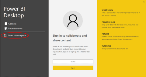
2. Select File – Open other reports from the splash dialog that appears upon entry, as shown.

Illustration 2: Select Open Other Reports on the Splash Dialog that Appears

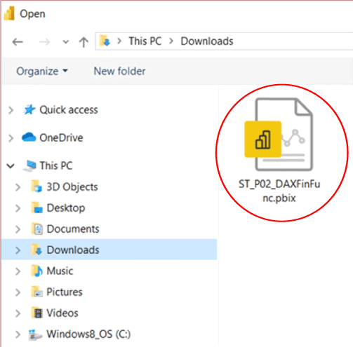
3. Navigate to the downloaded .pbix file.

Illustration 3: Select the Downloaded File and Open …

4. Click Open.

The .pbix file opens, and you arrive within the Report view, which consists of a single tab containing a blank canvas. As many of you are aware, you can tell you are in the Report view because the current view (of the three views available in the upper left corner, Report, Data, and Model) is indicated by the yellow bar to the left of the icon.

5. Click the Data view icon along the left of Power BI Desktop (underneath the Report view icon), as desired, to become familiar with the basic sample model, which includes three rows of asset data.

At this point, you’ll construct a table visualization to contain asset details, to which you will need to be able to easily add a depreciation calculation using a DAX financial function in the practice example for the first (Straight-line) depreciation type. This table will also serve as a model for practice examples for the subsequent depreciation functions.

Construct a Table Visualization to Contain Basic Asset Data

1. In the sample Power BI model, make sure to be in the Report view.
2. Click the cursor in the upper half of the blank canvas.
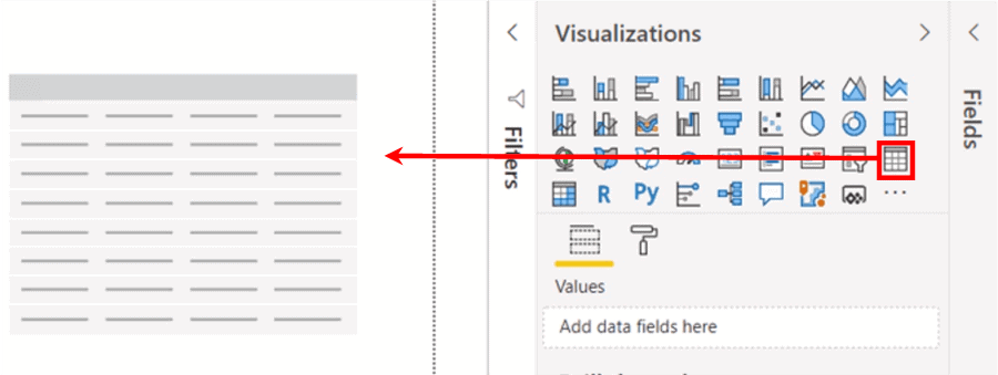
3. Click the Table icon in the collection atop the Visualizations tab, to create a blank table on the canvas.

Illustration 4: Create a New Table Visualization on the Canvas

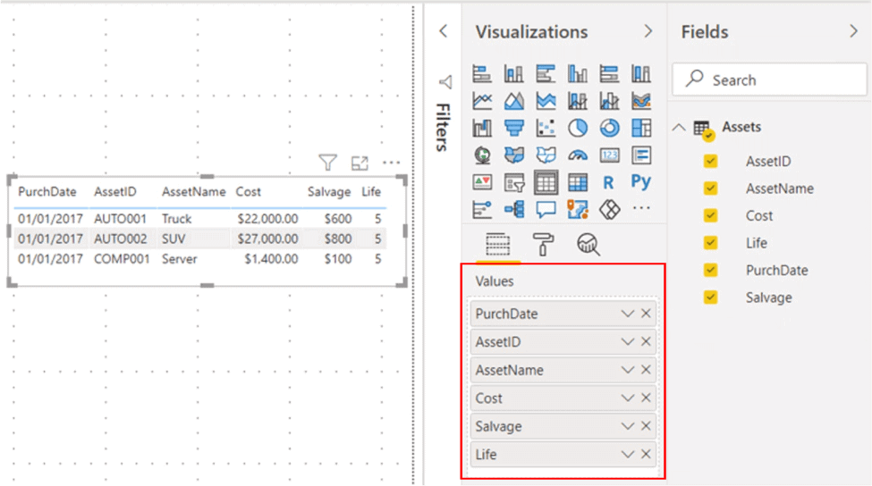
4. Ensuring that the above table visualization is selected, add the following fields (from the Assets table in the Fields pane) to the Values section of the Fields tab of the Visualizations pane:
   • PurchDate
   • AssetID
   • AssetName
   • Cost
   • Salvage
   • Life

The fields appear in the table as depicted.

Illustration 5: Additions in the Values Section of the Fields Tab

Finally, it’s a good idea to label the table you’re creating – as I’ve said throughout my Stairway to DAX and Power BI series and elsewhere. This is a minor point, but, as multiple visualizations tend to accumulate within a development environment, it’s often helpful to make them easily distinguishable via descriptive, “working” titles. It’s also a great way to identify the “at-a-glance” verification mechanism for other internal team members to use, say, in granting approval to promote a model and its contents to production from development.

5. With the new table selected, once again, click the Format (“paint roller”) tab, underneath the visualizations collection atop the Visualizations pane.
6. Scroll down to the Title section of the Format settings.
7. Click the Title slider to On.
8. Expand the Title section by clicking the carat to the left of the Title label.
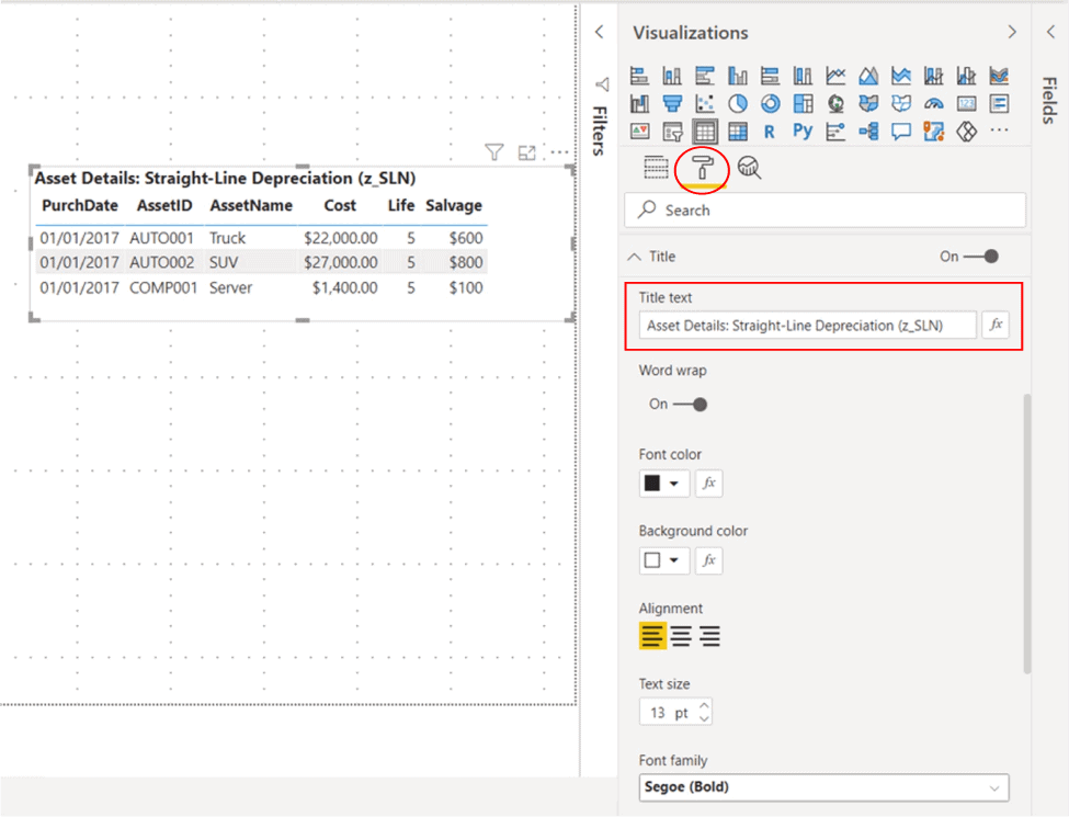
9. Type Asset Details: Straight-Line Depreciation (z_SLN) into the Title text box.
10. Set formatting as desired (you can see what I used in the illustration below).

The settings for the Title section of the Format tab appear, alongside the new table, somewhat as depicted.

Illustration 6: Title Settings for the New Table

You now have a basic Asset Depreciation table that will serve as a template container for each DAX depreciation function introduced throughout the practice session below. This will provide a combined view of the relevant factors involved in the use of each function, as well as a comparative look at the different values the calculations generated.

Before proceeding, you can speed preparation for the practice exercises by cloning a table similar to the one above for each of the three additional DAX depreciation functions we will be examining. The calculation set we create for every function taken up within this article (except for the Straight-line Depreciation function taken up first) generates a different depreciation value for each period, requiring a separate calculation for each period, as you’ll see. But the initial table you have created contains the “common core” of all the tables created in this article. And working with a set of clones of that table will be more efficient than creating all from scratch.

Create a “Clone” of the Table Visualization Created Above for Each of the Remaining DAX Depreciation Functions within the Practice Example

You can use a quick “copy and customize” approach to create a separate table to house each of your upcoming practice examples.

1. Click the table you created above on the canvas to select it.
2. Select CTRL+C (“Copy”) to copy the existing table visualization.
3. Click outside the table and onto the blank canvas.
4. Select CTRL + V (“Paste”) on the keyboard to create an identical copy of the table you just created.
5. Repeat Steps 3 and 4 above two more times, for a total of three times, to create three copies of the same table.

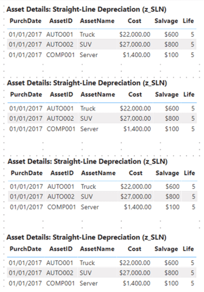
You now have four identical copies of the original table visualization.

6. Turn on Gridlines (under the View tab on the main menu) if you find it useful in arranging visualizations.
7. Move the newly created (at this point identical) copies to align them evenly, below the original, on the canvas, to create working space, approximately as shown.

Illustration 7: “Four Tables for Four Practice Sets:” Copies below the Original …

Now, all that remains is to customize each of the templates you have cloned so that the DAX depreciation function to be demonstrated in each is reflected in its title. The good news is that the existing title is already formatted, and needs only a modification in the description of the function it will contain, as you’ll see in the next steps.

1. With the second table from the top selected, click the Format tab, once again, underneath the visualizations collection atop the Visualizations pane.
2. Scroll down to the Title section of the Format settings, as you did earlier with the original table visualization created.
3. Expand the Title section by clicking the carat to the left of Title label, if necessary.
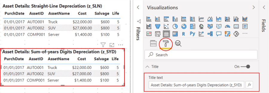
4. Change the Title from Asset Details: Straight-Line Depreciation (z_SLN) to Asset Details: Sum-of-years Digits Depreciation (z_SYD).
5. Leave formatting and other settings within the Title section as they were set in the original.

The second clone table now appears, above the original table, as depicted.

Illustration 8: The Second Clone Becomes the SYD Calculations Table …

You’ll next customize a table to house the Fixed Declining Balance calculation you will craft.

1. With the third table from the top selected, click the Format tab, once again, underneath the visualizations collection atop the Visualizations pane.
2. Scroll down to the Title section of the Format settings, as you did within each of the earlier two table visualizations.
3. Expand the Title section by clicking the carat to the left of Title label, as required.
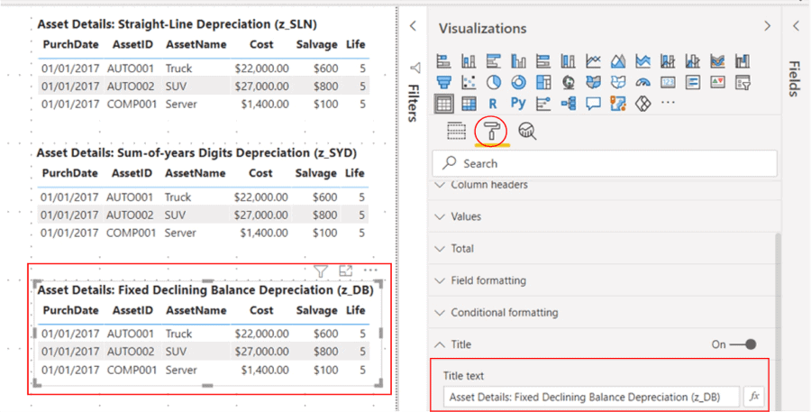
4. Change the Title from Asset Details: Straight-Line Depreciation (z_SLN) to Asset Details: Fixed Declining Balance Depreciation (z_DB).
5. Leave formatting and other settings within the Title section as set in the original.

The third clone table now appears, above the original table, as depicted.

Illustration 9: The Third Clone Becomes the DB Calculations Table …

Finally, you’ll create a table to house the Double-Declining Balance calculation you will write.

1. With the fourth table from the top selected, click the Format tab, as before, underneath the visualizations collection atop the Visualizations pane.
2. Scroll down to the Title section of the Format settings, as you did within each of the earlier three table visualizations.
3. Expand the Title section by clicking the carat to the left of Title label, as needed.
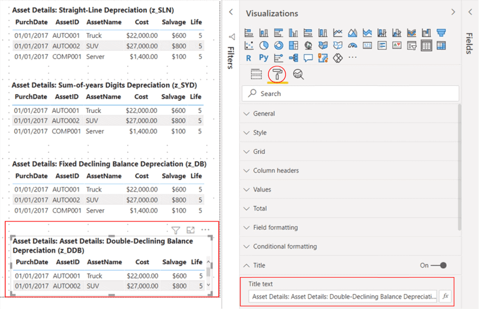
4. Change the Title from Asset Details: Straight-Line Depreciation (z_SLN) to Asset Details: Double-Declining Balance Depreciation (z_DDB).
5. Leave formatting and other settings within the Title section as set in the original.

The fourth clone table now appears, above the original table, as depicted.

Illustration 10: The Fourth Clone Becomes the DDB Calculations Table …

You’re now ready to begin putting the DAX depreciation functions to work within the practice steps for each below.

Shared Parameters for DAX Financial Functions for Depreciation

The financial functions introduced in this article all share the same objective: To support the computation of depreciation. While the accounting rules / assumptions contained within each function differ, they largely draw upon the same arguments / parameters as a basis upon which to apply their respective rules and calculate depreciation.

To gain an introduction to the operation of the functions efficiently, you’ll work through a separate practice exercise for each. Because the basic arguments share three common arguments, it makes sense to explain the shared arguments / parameters here, so as not to repeat them in the Syntax section of each function. Should you need to refresh your understanding of any given argument’s meaning, you need only refer to the below.

The shared arguments / parameters are:

• Cost – The initial cost of the asset. From a capitalization perspective, Cost typically includes purchase price, together with transportation / shipping, setup and preparation costs, taxes, etc. What can be included depends upon accounting / tax statutes, policies and procedures in effect for the owner.

• Salvage – The value at the end of the depreciation. Also known as the “salvage value” of the asset, this takes into account what the asset, at the end of its economic life, might still be worth, or sold / exchanged for.

Example: A truck that was initially put on a company’s books at $22,000, has reached the end of its economic life after five years, based upon organizational accounting and tax policy. At this time, the vehicle is determined to have a “blue book” / market value of $600, which might be described as the “remaining,” or “salvage” value.

• Life – The number of periods over which the asset is depreciated (sometimes called the “economic” or “useful” life of the asset).

You’ll work with the individual functions in the sections that follow.

DAX Financial Function: SLN()

According to the Data Analysis Expressions (DAX) Reference, the SLN() function “returns the straight-line depreciation of an asset for one period.”

Straight line depreciation is the simplest way of calculating the depreciation of an asset. The depreciation amount is the same (hence “straight-line) over each period of the asset’s life. SLN() returns the periodic depreciation allowance based upon the values you supply it.

Example: The truck mentioned earlier, put on a company’s books at $22,000, with a salvage value of $600 and a life of five years, would generate annual depreciation of $ 4,280 via the straight-line method. The SLN() function would calculate depreciation via the following logic:

Straight Line Depreciation = (Cost – Salvage) / Life = $ 21,400 / 5 yr. = $4,280 per year

Syntax

Syntactically, the parameters / arguments you provide are specified within the parentheses to the right of SLN() as shown:

SLN(<cost>, <salvage>, <life>)

The parameters are explained in the section named Shared Parameters for DAX Financial Functions for Depreciation above.

Return Value and Further Remarks

SLN() returns the straight-line depreciation for one period. Periodicity assumed within (and built into) the calculation, therefore, determines the periodicity of the output.

You’ll get some hands-on practice with SLN() in Power BI Desktop in the next section.

Practice

The operation of SLN() will become clear using the data contained in the Power BI model you have downloaded and prepared above. You’ll begin with the dataset that appears in the model, and create a calculation that employs SLN(), whose parameters are selected from the assets data in the table provided. Along with the other functions you examine in this article, the “answer” to be expected via the calculation you create will appear in the associated practice step of this section for easy comparison.

Employ the DAX SLN() Function to Generate Basic Periodic Depreciation Value

You can take the following steps to create a calculation to return basic periodic depreciation values within the sample dataset.

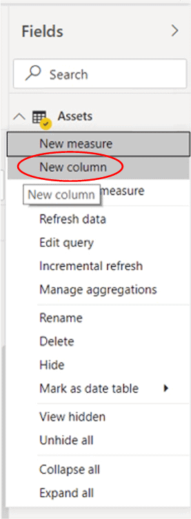
1. From the Report view, right-click the Assets table in the Fields pane of the model.
2. Select New column from the context menu that appears, as depicted.

Illustration 11: Creating a New Calculation …

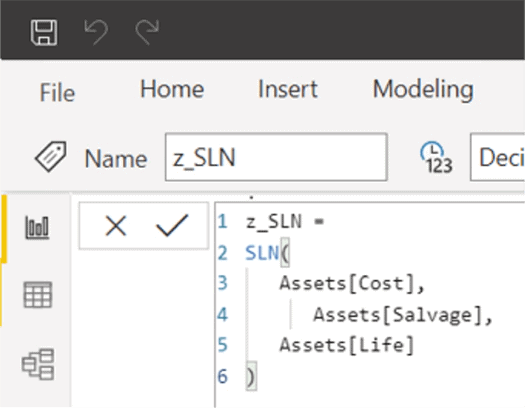
3. Type, or cut and paste, the following into the Formula bar:

z_SLN = 
SLN(
   Assets[Cost], 
      Assets[Salvage], 
   Assets[Life]
)

The calculation appears as shown in the Formula bar:

Illustration 12: Calculation Containing the SLN() Function …

4. Click the checkmark to the left of the Formula bar to check and commit the calculation, and to create the new calculated column.

The calculation z_SLN appears within the Assets table in the Fields pane.

NOTE: You will name the calculations you create in this article with a z_ prefix. This leaves their names very close to that of the DAX financial function they employ, while making them easily identifiable (via a separate physical grouping) from the base model columns. Other methods of grouping calculations are, of course, available.

5. With the new calculated column z_SLN selected in the Fields pane, make the following Format settings underneath the main menu:
   • Currency ($)
   • 2 decimal places
   • Don’t summarize

Illustration 13: Calculated Column Format Settings

6. Select the Asset Details: Straight-Line Depreciation (z_SLN) table visualization, once again, and then click the checkbox to the left of the new z_SLN calculation. To add it to the Values section of the Fields tab for the table, underneath the existing Life column.

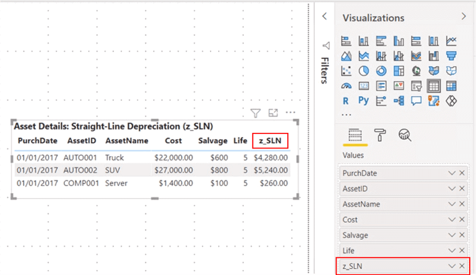
The z_SLN value within the Loan Details table visualization appears as shown. This can serve as a means of checking the output accuracy of the new calculation within your own Power BI Desktop model.

Illustration 14: Straight-line Depreciation Value Returned via the New Calculation

If you’ve obtained similar results to the above, you can conclude that you’ve successfully assembled a calculation to demonstrate the operation of the DAX SLN() financial function.

Straight-line depreciation makes sense to even non-accountants, assuming the concept of depreciation itself, etc., does not present an obstacle. The remaining modes of depreciation, three functions for which we will consider in the following sections, manipulate (for accounting and tax, as well as other reasons) the depreciation charged per period. This manipulation typically is driven by a need / option to accelerate depreciation or influence the rate at which the depreciation is charged – often resulting from tax considerations. A light overview of each method will be included in the discussion of each, but abundant information is available online, at the IRS and state taxing authority sites, etc., if this is of interest.

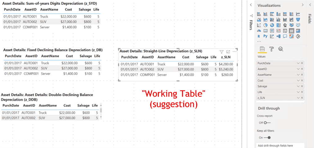
NOTE: As a tip, you may find it convenient to move the other three practice calculation tables to the left of the “table in play,” while working with any given depreciation calculation in this article – something like the arrangement shown below. You can always move things around to match what you see in the working illustrations at any given point in the practice steps.

Illustration 15: Suggested Arrangement of Working vs. Non-Working Tables in Sample Practice Exercise

Keep in mind, as you lay out your tables, that all except the first table (housing SLN() function) will have multiple additional columns, as the respective period calculation will generate a separate value, hence column, for each of the five years presented in the corresponding table visualization.

In the next section, you’ll be introduced to the DAX SYD() depreciation function.

DAX Financial Function: SYD()

According to the Data Analysis Expressions (DAX) Reference, the SYD() function “returns the sum-of-years’ digits depreciation of an asset for a specified period.” SYD() is a popular accelerated depreciation function, providing support for reducing the calculated value of an asset by a larger amount during the first period of its lifetime, and successively smaller amounts during subsequent periods.

Sum-of-years’ Digits Method: The Concepts

The sum-of-years’ digits depreciation technique accelerates depreciation based upon the assumption that assets are generally more productive when they are new, and that their productivity (and hence economic value) decreases as they become old. An example will likely help illustrate the mechanical steps behind the technique:

Example: The truck mentioned earlier, put on a company’s books at $22,000, with a salvage value of $600 and a life of five years, would have generated annual depreciation of $ 4,280 via the straight-line method.

The SYD() function would calculate depreciation via the following logic:

1. Determine the years’ digits value: Since the asset has a useful life of 5 years, the years’ digits are: 5, 4, 3, 2, and 1. The sum of the digits is 5+4+3+2+1=15.

NOTE: The sum of the digits can also be determined by using the formula (n2+n)/2 where n is equal to the useful life of the asset in years. The example would be shown as (52+5)/2=15

2. Depreciable base = Cost − Salvage value
3. SYD depreciation = Depreciable base x (Remaining useful life / Sum of the years’ digits)
4. Calculate depreciation rates for each period of life:

1. • 5/15 for the 1st year
   • 4/15 for the 2nd year
   • 3/15 for the 3rd year
   • 2/15 for the 4th year
   • 1/15 for the 5th year

Depreciation expense by respective period (year) would be generated as follows:

Period (Year)	Depreciable Base	Depreciation Rate	Depreciation Expense
1	$ 21,400	5/15	$ 7,133.33
2	$ 21,400	4/15	$ 5,706.67
3	$ 21,400	3/15	$ 4,280.00
4	$ 21,400	2/15	$ 2,853.33
5	$ 21,400	1/15	$ 1,426.67
Total			$21,400.00 ( $ 600 scrap value remains)

Table 1: Depreciation by Period via the Sum-of-years’ Digits Method

The point here is to illustrate what goes on behind the scenes when you use the DAX SYD() function. Understanding the mechanics can make it easier to intelligently select and use the function as required in the business environment, particularly when you identify the method from an examination of existing depreciation reports, built within, say, MS Excel, where the function is very similar.

Syntax

Syntactically, the parameters / arguments you provide are specified within the parentheses to the right of SYD() as shown:

SYD(<cost>, <salvage>, <life>, <per>)

The arguments common to the DAX depreciation functions as a group are explained in the section named Shared Parameters for DAX Financial Functions for Depreciation above. The Per parameter, relevant to this function, does not occur in all DAX depreciation functions.

Per – The period for which you wish to calculate depreciation. Must use the same units as Life, with a value between 1 and Life (inclusive).

Return Value and Further Remarks

The DAX SYD() function returns the Sum-of-years’ digits depreciation for the specified period. Periodicity assumed in the calculation therefore determines periodicity of the output.

You’ll get some hands-on practice with SYD() in Power BI Desktop in the next section.

Practice

The operation of SYD() will become clear using the data contained in the Power BI model you have downloaded and prepared above. You’ll begin with the dataset that appears in the model, once again, and create calculations that employ SYD(), whose parameters are selected from the assets data in the table provided. Along with the other functions you examine in this article, the “answer” to be expected via the calculations you create will appear in the associated practice step of this section for easy comparison.

Employ the DAX SYD() Function to Generate Sum-of-years’ Digits Depreciation Values

You can take the following steps to create a calculation to generate Sum-of-years’ Digits depreciation values for each of the years of the lives of the assets in the practice data set.

Create Five Separate SYD() Calculations, One for Each Year of Asset Life

1. From the Report view, right-click the Assets table in the Fields pane of the model.
2. Selecting New column from the context menu that appears, as you did within the earlier calculation, and following the steps you took in creating a calculation there, create the following five calculations within the Assets table of the model:

Calculation Name	Calculation Syntax
z_SYD-2017	z_SYD-2017 = SYD( Assets[Cost], Assets[Salvage], Assets[Life],1 )
z_SYD-2018	z_SYD-2018 = SYD( Assets[Cost], Assets[Salvage], Assets[Life],2 )
z_SYD-2019	z_SYD-2019 = SYD( Assets[Cost], Assets[Salvage], Assets[Life],3 )
z_SYD-2020	z_SYD-2020 = SYD( Assets[Cost], Assets[Salvage], Assets[Life],4 )
z_SYD-2021	z_SYD-2021 = SYD( Assets[Cost], Assets[Salvage], Assets[Life],5 )

Table 2: Sum-of-years’ Digits Method Calculations to Add to the Assets Table

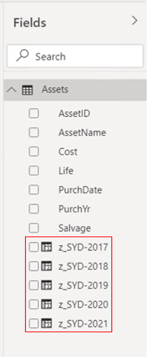
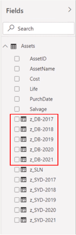
The calculations appear in the Fields pane, Assets table, as depicted.

Illustration 16: z_SYD Calculations in the Fields Pane

NOTE: Approaches vary, of course, for grouping calculations and, in the business environment, placing them in a folder, etc., might have organizational advantages. For purposes of this set of practice exercises, however, you’ll keep them in simple groups via the z_ prefix as shown.

3. For each new calculated column in the z_SYD group, select the calculation and make the following Format settings (Column tools menu):
   • Currency ($)
   • 2 decimal places
   • Don’t summarize
   •  

Illustration 17: Example z_SYD Member Calculated Column Format Settings (Column Tools)

4. Ensuring that the Asset Details: Sum-of-years Digits Depreciation (z_SYD) table visualization is selected, add the new z_SYD calculations to the Values section of the Fields tab for the table, underneath the existing Life column.

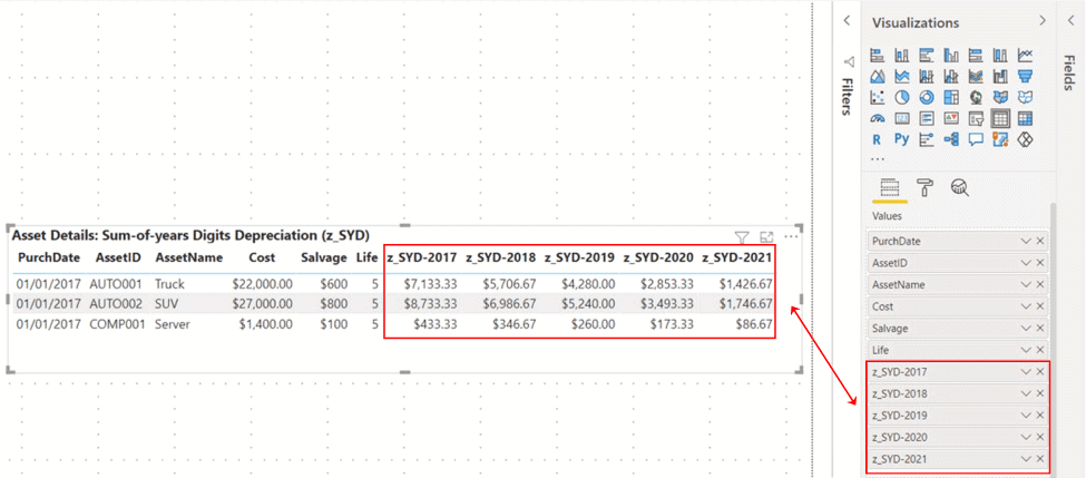
The five, newly added z_SYD values, each generating the depreciation charged to the respective period year, appear within the Asset Details: Sum-of-years Digits Depreciation (z_SYD) table visualization as shown. This can serve as a means of checking the output accuracy of the new calculation within your own Power BI Desktop model.

Illustration 18: SYD Depreciation Value for Respective Year Returned via the New Calculations

Once again, if you’ve obtained similar results to the above, you can conclude that you’ve successfully assembled the calculations to demonstrate the operation of the DAX SYD() financial function over the lives of assets with the characteristics described in the data.

In the next section, you’ll be introduced to the DAX DB() depreciation function.

DAX Financial Function: DB()

According to the Data Analysis Expressions (DAX) Reference, the DB() function “returns the depreciation of an asset for a specified period using the fixed-declining balance method.” DB() is another popular accelerated depreciation function, providing support, once again, for reducing the calculated value of an asset by a larger amount during the first period of its lifetime, and smaller amounts during subsequent periods.

Fixed Declining Balance Method: The Concepts

The Fixed Declining Balance depreciation technique, like the Sum-of-years Digits (SYD() ) function I introduced in the section immediately previous, assumes that assets are generally more productive when they are new and their productivity / economic value decreases as they become old. An example, once again, may help illustrate the mechanics for the Fixed Declining Balance technique:

Example: The truck mentioned earlier, put on a company’s books at $22,000, with a salvage value of $600 and a life of five years, would have generated annual depreciation of $ 4,280 via the straight-line method.

The DB() function would calculate depreciation via the following logic:

1. Depreciable Base = Cost – Accumulated Depreciation Deduct the Depreciation Expense taken to date, from the beginning cost of the asset (in this case, do not deduct Salvage Value, which is taken into consideration within the Depreciation Rate).
2. Depreciation Rate = 1− ((Salvage / Cost) ^{(1 / Life)} (Rounded to three decimal places within the DB() function, and fairly common within accounting and finance references). This rate remains the same for each year of asset life within the Fixed Declining Balance depreciation technique, with special case consideration for first and last periods where the first period is not a full twelve months. For more information, see the Data Analysis Expressions (DAX) Reference for the DB() function.

Depreciation expense for the cited example, by respective period (year), would be generated as follows:

Period (Year)	Depreciable Base	Depreciation Rate	Depreciation Expense
1	$ 22,000.00	0.513	$ 11,286.00
2	$ 10,714.00	0.513	$ 5,496.28
3	$ 5,217.72	0.513	$ 2,676.69
4	$ 2,541.03	0.513	$ 1,305.55
5	$ 1,237.48	0.513	$ 634.83
Total			$21,400.00 ( $ 600 scrap value remains, plus small rounding difference)

Table 3: Depreciation by Period via the Fixed Declining Balance Method

Once again, the idea is to illustrate what transpires within the DAX DB() function. In most cases, the business environment will stipulate, via accounting / finance / tax considerations the depreciation policies – and hence the specific method that will drive the DAX function you select for a given task. However, it certainly helps to understand what is going on “under the covers” in cases when, say, a Power BI visualization is returning unexpected results.

Syntax

Syntactically, the parameters / arguments you provide are specified within the parentheses to the right of DB() as shown:

DB(<cost>, <salvage>, <life>, <period>[, <month>])

As you’ve already discovered, the arguments common to the DAX depreciation functions as a group are explained in the section named Shared Parameters for DAX Financial Functions for Depreciation above. The Period and Month (where applicable) parameters, relevant to this function, do not occur in all DAX depreciation functions.

Period – The period for which you wish to calculate depreciation. It must use the same units as Life, with a value between 1 and Life (inclusive).

Month – (Optional) The number of months in the first year. If the month is omitted, it is assumed to be 12.

Return Value and Further Remarks

The DAX DB() function returns the Fixed Declining Balance depreciation for the specified period.

You’ll get some hands-on practice with DB() in Power BI Desktop in the next section.

Practice

As with the earlier depreciation functions in the previous exercises, operation of DB() will become clear using the data contained in the Power BI model you have downloaded and prepared above. You’ll begin with the dataset that appears in the model, once again, and create calculations that employ DB(), whose parameters are selected from the assets data in the table provided. Along with the other functions you examine in this article, the “answer” to be expected via each calculation you create will appear in the associated practice step of this section for easy comparison.

Employ the DAX DB() Function to Generate Fixed Declining Balance Depreciation Values

You can take the following steps to create a calculation to generate Fixed Declining Balance depreciation values for each of the years of the lives of the assets in the practice data set.

Create Five Separate DB() Calculations, One for Each Year of Asset Life

1. From the Report view, right-click the Assets table in the Fields pane of the model.
2. Selecting New column from the context menu that appears, as you did within the calculations created for earlier practice exercise steps of this article, and following the steps you took in creating a calculation there, create the following five calculations within the Assets table of the model:

Calculation Name	Calculation Syntax
z_DB-2017	z_DB-2017 = DB( Assets[Cost], Assets[Salvage], Assets[Life],1 )
z_DB-2018	z_DB-2018 = DB( Assets[Cost], Assets[Salvage], Assets[Life],2 )
z_ DB-2019	z_DB-2019 = DB( Assets[Cost], Assets[Salvage], Assets[Life],3 )
z_ DB-2020	z_DB-2020 = DB( Assets[Cost], Assets[Salvage], Assets[Life],4 )
z_ DB-2021	z_DB-2021 = DB( Assets[Cost], Assets[Salvage], Assets[Life],5 )

Table 4: Fixed Declining Balance Method Calculations to Add to the Assets Table

The calculations appear in the Fields pane, Assets table, as depicted.

Illustration 19: z_DB Calculations in the Fields Pane

3. For each new calculated column in the z_DB group, select the calculation and make the following Format settings (Column tools menu), as done with calculations in previous sections.
   • Currency ($)
   • 2 decimal places
   • Don’t summarize
4. Ensuring that the Asset Details: Fixed Declining Balance Depreciation (z_DB) table visualization is selected, add the new z_DB calculations to the Values section of the Fields tab for the table, underneath the existing Life column.

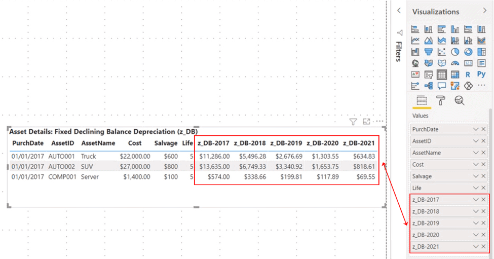
The five, newly added z_DB values, each generating the depreciation charged to the respective period year, appear within the Asset Details: Fixed Declining Balance Depreciation (z_DB) table visualization as shown. This can serve as a means of checking the output accuracy of the new calculation within your own Power BI Desktop model.

Illustration 20: DB() Depreciation Value for Respective Year Returned via the New Calculations

If you’ve obtained similar results to the above, you can conclude that you’ve successfully assembled the calculations to demonstrate the operation of the DAX DB() financial function over the lives of assets with the characteristics described in the data.

In the next section, you’ll be introduced to the DAX DDB() depreciation function.

DAX Financial Function: DDB()

According to the Data Analysis Expressions (DAX) Reference, the DDB() function “returns the depreciation of an asset for a specified period using the double-declining balance method or some other method you specify.” DDB() is yet another depreciation function that provides support for reducing the calculated value of an asset is by a larger amount during the first period of its lifetime, and smaller amounts during subsequent periods.

Double Declining Balance Method: The Concepts

The Double Declining Balance depreciation technique shares a basic concept with other accelerated depreciation techniques – like the Sum-of-years Digits (SYD()) and the Fixed Declining Balance (DB()) financial functions I introduced in the earlier sections: The Double Declining Balance technique assumes higher productivity in newer assets, and waning productivity / economic value as assets age.

The Double Declining Balance technique, in the simplest scenario, doubles the Straight-line rate and multiples it times the book value (Cost – Accumulated Depreciation) at the beginning of the respective period.

There are a couple of twists that you might not expect with the Double Declining Balance depreciation technique – factors that reflect the traditional technique as consistently practiced within the accounting / finance context and which are reflected within the DAX DDB() financial function:

• The first thing that has confused some early adopters is a matter of the naming of the method: They have assumed, from the outset that “Double Declining Balance” simply means “two times the period depreciation generated by the Fixed Declining Balance method. This assumption reveals itself to be faulty early in the attempt to apply it in an understanding of the Double Declining Balance technique, but it might save some time to learn about the actual workings of the technique before getting started with a partial understanding.
• The Double Declining Balance calculation does not consider the salvage value in the depreciation of each period. Where book value falls below the salvage value, the last period would likely be adjusted so that it ends at the salvage value. This might need to be taken into consideration if you are, say, constructing a visualization / report involving the DDB() function, and are expecting the total of the depreciation expenses over the periods of the life of the asset to net out to precisely the economic value (cost-less-salvage value) at the end of the asset life. While a simple plug could be constructed in Power BI / other reporting mechanisms, it would be best to consult accounting / finance on the best way to handle this in your own environment. (A variable declining balance approach might be an alternative option.)

An example may help illustrate the mechanics for the Double Declining Balance technique:

Example: The truck mentioned earlier, put on a company’s books at $22,000, with a salvage value of $600 and a life of five years, would have generated annual depreciation of $ 4,280 via the straight-line method.

The DDB() function would calculate depreciation via the following logic:

1. Straight-Line Depreciation Percent = 100 % / Economic Life Simply generate an annual depreciation percent.
2. Depreciation Rate = 2 x Straight-Line Depreciation Percent The “double” in “Double-Declining Balance”
3. Depreciation for a Period = Depreciation Rate x Depreciable Base at Beginning of the Period Depreciation expense for the cited example, by respective period (year), would be generated as follows:

Period (Year)	Depreciable Base	Depreciation Rate	Depreciation Expense
1	$ 22,000.00	.400	$ 8,800.00
2	$ 13,200.00	.400	$ 5,280.00
3	$ 7,920.00	.400	$ 3,168.00
4	$ 4,752.00	.400	$ 1,900.80
5	$ 2,851.20	.400	$ 1,140.48
Total			$ 20,289.28 ( $ 600 scrap value remains, plus $ 1,110.72 difference – to be handled via accounting, etc., adjustment, as discussed above)

Table 5: Depreciation by Period via the Double Declining Balance Method

As before, the idea is to illustrate what transpires within the DAX DDB() function. It is important to always keep in mind that the business environment will stipulate, via accounting / finance / tax considerations, the depreciation policies – and hence the specific method – that will drive the DAX function you select for a given task, as I have stated already.

Syntax

Syntactically, the parameters / arguments you provide are specified within the parentheses to the right of DDB() as shown:

DDB(<cost>, <salvage>, <life>, <period>[, <factor>])

The arguments common to the DAX depreciation functions as a group are explained in the section named Shared Parameters for DAX Financial Functions for Depreciation above. The Period and Factor (where applicable) parameters, relevant to this function, do not occur in all DAX depreciation functions.

Period – The period for which you wish to calculate depreciation. Must use the same units as Life, with a value between 1 and Life (inclusive).

Factor – (Optional) The rate at which the balance declines. If factor is omitted, it is assumed to be 2 (the Double Declining Balance method).

Return Value and Further Remarks

The DAX DDB() function returns the Double Declining Balance depreciation for the specified period.

You’ll get some hands-on practice with DDB() in Power BI Desktop in the next section.

Practice

As has been the case with the depreciation functions in the previous exercises, using the data contained in the Power BI model you have downloaded and prepared above will help to clarify and activate what you’ve learned about the operation of DDB() to this point. You’ll begin with the dataset that appears in the model, once again, and create calculations that employ DDB(), whose parameters are selected from the assets data in the table provided. And, as you have done with the other functions you’ve examined in this article, the “answer” to be expected via each calculation you create will appear in the associated practice step of this section for easy comparison.

Employ the DAX DDB() Function to Generate Double Declining Balance Depreciation Values

You can take the following steps to create a calculation to generate Double Declining Balance depreciation values for each of the years of the lives of the assets in the practice data set.

Create Five Separate DDB() Calculations, One for Each Year of Asset Life

1. From the Report view, right-click the Assets table in the Fields pane of the model.
2. Selecting New column from the context menu that appears, as you did within the calculations created for earlier practice exercise steps of this article, and following the steps you took in creating a calculation there, create the following five calculations within the Assets table of the model:

Calculation Name	Calculation Syntax
z_DDB-2017	z_DDB-2017 = DDB( Assets[Cost], Assets[Salvage], Assets[Life],1 )
z_DDB-2018	z_DDB-2018 = DDB( Assets[Cost], Assets[Salvage], Assets[Life],2 )
z_DDB-2019	z_DDB-2019 = DDB( Assets[Cost], Assets[Salvage], Assets[Life],3 )
z_DDB-2020	z_DDB-2020 = DDB( Assets[Cost], Assets[Salvage], Assets[Life],4 )
z_DDB-2021	z_DDB-2021 = DDB( Assets[Cost], Assets[Salvage], Assets[Life],5 )

Table 5: Double Declining Balance Method Calculations to Add to the Assets Table

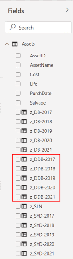
The calculations appear in the Fields pane, Assets table, as depicted.

Illustration 21: z_DDB() Calculations in the Fields Pane

4. For each new calculated column in the z_DDB() group, select the calculation and make the following Format settings (Column tools menu), as done with calculations in previous sections.
   • Currency ($)
   • 2 decimal places
   • Don’t summarize
5. Ensuring that the Asset Details: Double Declining Balance Depreciation (z_DDB()) table visualization is selected, add the new z_DDB() calculations to the Values section of the Fields tab for the table, underneath the existing Life column.

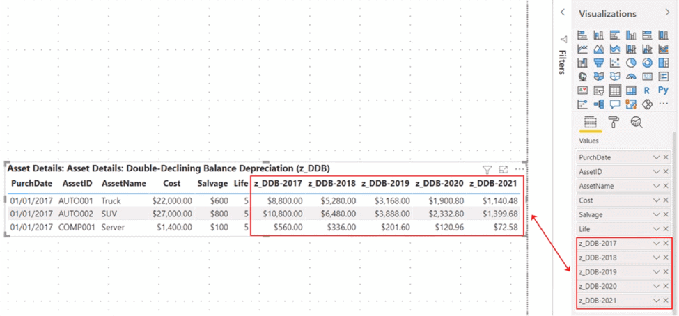
The five, newly added z_DDB() values, each generating the depreciation charged to the respective period year, appear within the Asset Details: Double Declining Balance Depreciation (z_DDB()) table visualization as shown. This can serve as a means of checking the output accuracy of the new calculation within your own Power BI Desktop model.

Illustration 22: DDB() Depreciation Value for Respective Year Returned via the New Calculations

As with the previous depreciation functions within this article, if you’ve obtained similar results to the above for DDB(), you can conclude that you’ve successfully assembled the calculations to demonstrate the operation of this financial function over the lives of assets with the characteristics described in the data.

Final Arrangement for Comparison of the DAX Depreciation Functions

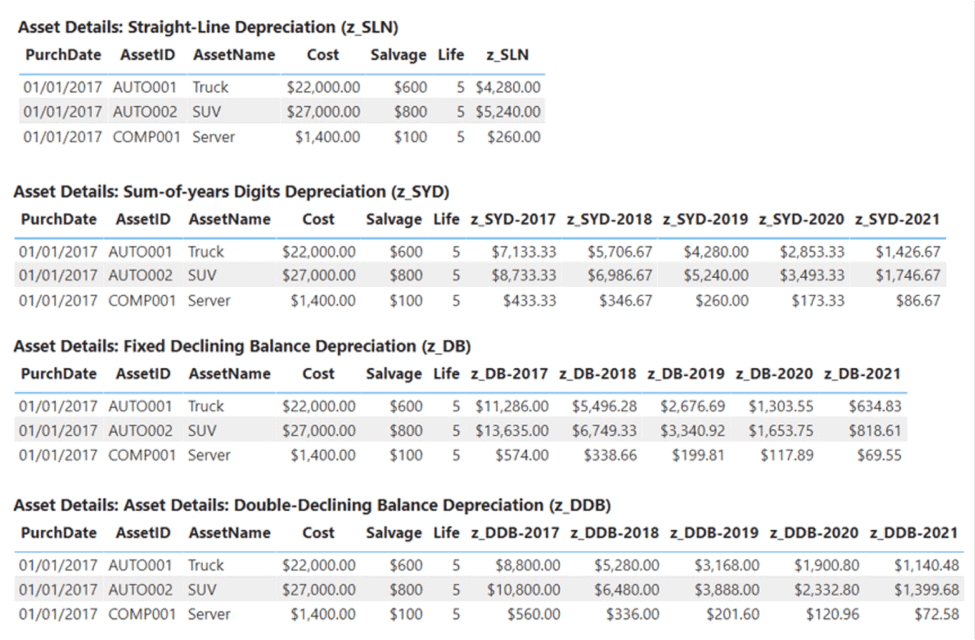
Now that you’ve finished creating a set of similar tables, within a single Power BI model, that generate depreciation with each DAX depreciation function respectively, you might want to arrange these tables for easy comparison of the outputs of these functions. While you may have a specific approach in mind for designing your own arrangement, you will find that this can easily be done by taking steps similar to those that follow.

Arrange the Tables Housing the Individual DAX Depreciation Functions to Permit Easy Comparison

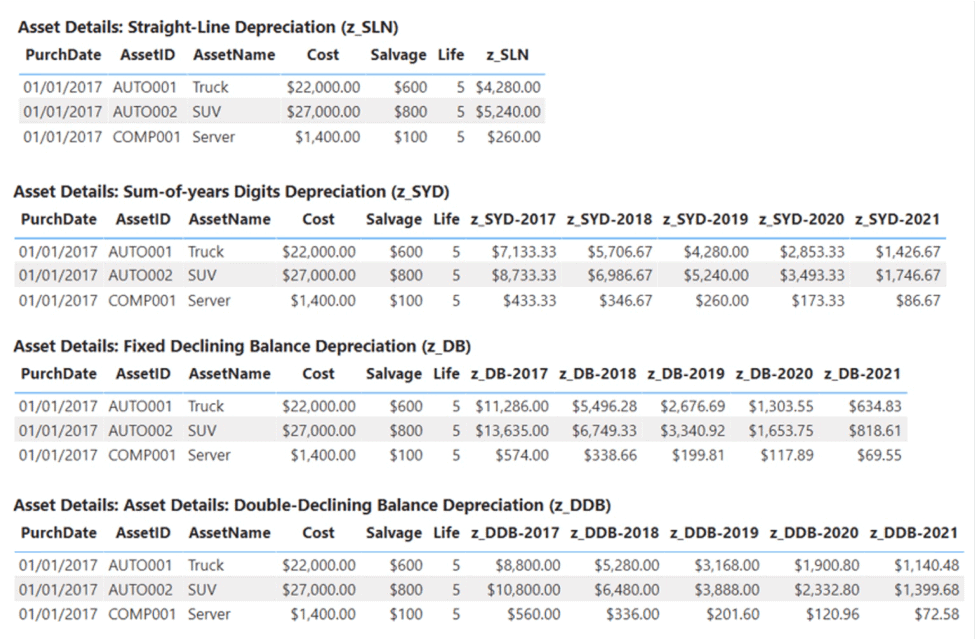
You can adjust sizing on the four tables you have created within the practice exercises, and then align / stack them atop each other to achieve an arrangement somewhat as shown.

Illustration 23: A Suggested Re-arrangement of the DAX Depreciation Tables

You might prefer to show only one table, based upon the exact choices of depreciation method made in the business environment, of course, or perhaps based upon parameterization to support the examination of the output of different method selections, or other variable values, at runtime. These and other options are, of course, easily accommodated with Power BI.

Summary

In this, second of a group of articles overviewing the new DAX financial functions, I introduced another popular subgroup of those functions that focuses upon depreciation. My objective was to examine how each function can be employed, within Power BI, to support analysis and reporting of the sort one might accomplish using Microsoft Excel. For each function you explored, you learned its purpose, then examined the DAX syntax involved in its use. Moreover, you gained exposure, via an illustrative example for each function, used the respective function with practice assets data, and then confirmed your understanding of the results you had obtained with each function.

 

The post DAX financial functions: Depreciation calculations appeared first on Simple Talk.

from Simple Talk https://ift.tt/3hEZbdw
via

PASS is Dead – Long Life to SQLFamily

This new year start with the death of PASS, the professional association that for so many years supported the SQLFamily around the world and helped so many to achieve their professional goals.

You can still read the communication, but PASS is ‘going dark’ on January 15, meaning none of its features and resources will be available after this date.

How can we keep the community together?

Challenging times result in tough people. The SQLFamily is tough and is proving it creating many replacements to keep the community together and making this in an organized way. Check the new meeting points and resources for the SQLFamily:

Microsoft

Microsoft announced they will provide some resources for SQL Server User Groups. All PASS User Groups should fill the form with Microsoft and wait for further communication.

The resources will be very welcome. I’m not a rooter of meetup communities, all of them I saw usually are very passive, without much interaction. Even so, it will be very welcome.

Data Saturdays

PASS holds the SQL Saturday name, we can’t create more SQL Saturdays. However, we only need to change the name and a big step was made by the community to replace SQL Saturdays with Data Saturdays.

The Data Saturday website is already online and announcing the next events. The site is open source and has a repository in github where everyone can contribute with new features for the site.

 I asked for an event myself, it will be the first Malta Data Saturday!

Hosting for Groups

SQLUGS provides hosting for user groups, you only need to ask. It’s a great way to replace the websites provided by PASS and it’s free

Data Community

The Data Community portal helps to spread the world about community events and it’s an interesting possible replacement to PASS. It also has a github repository, although I’m not sure if it is complete.

Call For Data Speakers

As the name implies, it’s a website to make speakers and event organizers meet themselves and discover the events around the community

Call For Speakers Facebook Group

A facebook group exclusive for speakers and event organizers to announce CfS’s 

Online Services

There are many online services available to help user group leaders to replace the resources provided by PASS. Here are some of them:

EventBrite: It’s great to create event registrations and announce events

Sessionize: This website was already becoming very common among the SQLFamily. When PASS announced it will be going dark on January 15, Sessionize included a new feature: Speakers can now search for events.

On a side note, the Data Saturdays are being built using EventBrite and Sessionize.

Meetup: Most user groups had their members registered with PASS. They have until January 15 to create other ways to register their members and invite everyone who is registered with PASS to register with the local group. Many groups are using meetup for this. The meetup is a paid service. The free version only allows 50 members.

Mailchimp: This is a great tool to create newsletters to the registered user group members, however, it can’t be used alone. It will require a facebook group or whatsApp group, some other online resource to keep the members in touch and interacting.

Conclusion

The SQLFamily is replacing PASS resources very fast and this is great. There is even some overlap on the sites and services created.

I hope this blog post can be useful as a reference point for the community and to help everyone expose their ideas on the comments and work to merge all solutions in a service to provide the user groups need.

Probably I forgot many other resources from the community, please, remind me on the comments.

 

The post PASS is Dead – Long Life to SQLFamily appeared first on Simple Talk.

from Simple Talk https://ift.tt/2L3FSP9
via