Tuesday, January 19, 2021

Power BI reading Parquet from a Data Lake

Data Lakes are becoming more usual every day and the need for tools to query them also increases.

While writing about querying a data lake using Synapse, I stumbled upon a Power BI feature I didn’t know was there.

When reading from a data lake, each folder is like a table. We store in the folder many files with the same structure, each file containing a piece of the data.

Data Lake tools are prepared to deal with the data on this way and read the files transparently for the user, but Power BI required us to read one specific file, not the folder. That’s until last November. If we google (verb: To google) about Power BI and Parquet files we can find many work arounds to read Parquet files in Power BI, but no mention to the new Parquet connector released on last November (https://powerbi.microsoft.com/en-us/blog/whats-new-in-power-query-dataflows-november-2020/), so I had to write about it.

The feature I’m illustrating on this article is in fact a combination of two features:

  • The feature to combine multiple files from Azure Data Lake Gen 2 storage. This was in preview in October 2019 in is available for a while, but I was surprised I couldn’t find any article really explaining the M code used to combine the files and how to customize the code.
  • The Parquet connector is the responsible to read Parquet files and adds this feature to the Azure Data Lake Gen 2. This connector was released in November 2020.

In order to illustrate how it works, I provided some files to be used in an Azure Storage. You can download the files here. You will also need to provision a new storage account and it will need to be an Azure Data Lake Storage Gen 2.

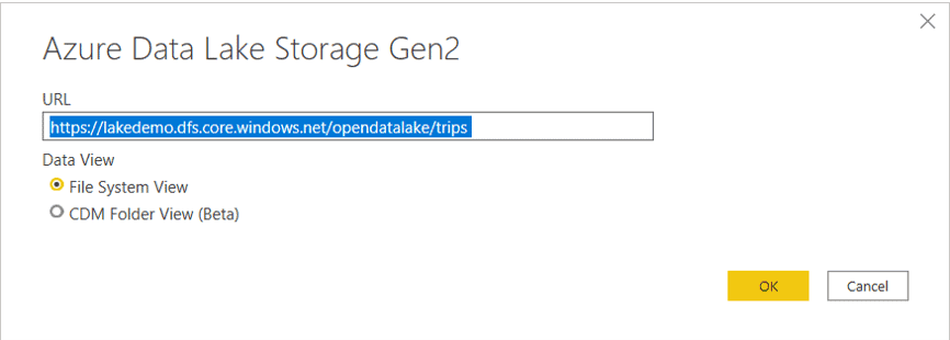
On the examples, I will use the address https://lakedemo.dfs.core.windows.net/opendatalake/trips for the storage, but you need to replace it with the DFS endpoint of your own storage.

Let’s make a step-by step:

  1. Open Power BI
  2. Select Get Data option on the main screen
  3. Select Azure Data Lake Storage Gen2. We will test directly with one of the most efficient options
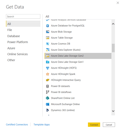
There are 3 storage options:

  • Azure Blob Storage
  • Data Lake Storage Gen 1
  • Azure Data Lake Storage Gen 2

It’s important to choose the correct option according your storage type, this affects the performance.

  1. On the URL box, type this URL: https://lakedemo.dfs.core.windows.net/opendatalake/trips
Graphical user interface, text, application Description automatically generated

  1. Click Ok button
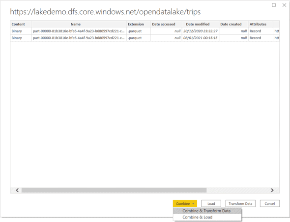
  2. Click the Combine button

Graphical user interface, text, application Description automatically generated

This screen has the traditional Transform and Load buttons but also has the Combine button, which has both options, Transform and Load, below it.

The traditional Transform and Load will be dealing with the list of files inside the Azure Storage folder. From this point, it will be our decision what to do with each file.

The Combine button, on the other hand, will bring to us a pre-built M script to combine all the files in the folder. It’s easy to mistake this feature believing Power BI will read only the current files, but in fact the script is flexible in such a way to read all the files in the folder, even future files included there.

  1. Select the option Combine & Transform
  2. Click Transform Data button

The M Code – How it Works

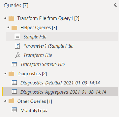
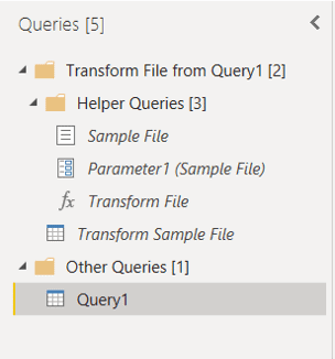
On Power Query window, you may notice the pre-built steps in the Applied Steps window. It’s also very interesting the way the queries were built: The final query is in a folder called Other Queries while you also have a folder called Helper Function containing a parameterized function.
Graphical user interface, application, Word Description automatically generated

Let’s analyze the M code to better understand how it works. Using the menu View-> Advanced Editor you can access the M code.

This is how our M code looks like:

let
  Source = AzureStorage.DataLake(“https://ift.tt/38T4pQ3;),
  #”Filtered Hidden Files1″ = Table.SelectRows(Source, each [Attributes]?[Hidden]? <> true),
  #”Invoke Custom Function1″ = Table.AddColumn(
    #”Filtered Hidden Files1″,
    “Transform File”,
    each #”Transform File”([Content])
  )
,
  #”Renamed Columns1″ = Table.RenameColumns(#”Invoke Custom Function1″, {“Name”, “Source.Name”}),
  #”Removed Other Columns1″ = Table.SelectColumns(
    #”Renamed Columns1″,
    {“Source.Name”, “Transform File”}
  )
,
  #”Expanded Table Column1″ = Table.ExpandTableColumn(
    #”Removed Other Columns1″,
    “Transform File”,
    Table.ColumnNames(#”Transform File”(#”Sample File”))
  )
,
  #”Removed Columns” = Table.RemoveColumns(#”Expanded Table Column1″, {“Source.Name”}),
  #”Grouped Rows” = Table.Group(
    #”Removed Columns”,
    {“Month”},
    {{“Trips”, each List.Sum([Trips]), type number}}
  )

in

  #”Grouped Rows”

These are the steps this code is executing:

  • Filter all files, making sure to not include hidden files
  • Use the AddColumn method to call the function “Transform File” for each row
  • Remove additional columns, leaving only the file name and result of the function
  • Expands the column containing the result of the function

This main script calls the Transform File function for each file in the folder. There is no fixed file name, all the files will be transformed and returned. This means that at any time new files are included in this data lake folder, a simple refresh will bring the data to the dashboard, leaving the solution flexible as a client solution for a data lake needs to be.

The M code for the Transform File function is this:

let
    Source = Parquet.Document(Parameter1),
    #”Changed Type” = Table.TransformColumnTypes(Source,{{“DateID”, type text}}),
    #”Added Custom” = Table.AddColumn(#”Changed Type”, “Month”, each Text.Middle([DateID],4,2)),
    #”Grouped Rows” = Table.Group(#”Added Custom”, {“Month”}, {{“Trips”, each Table.RowCount(_), Int64.Type}}),
    #”Changed Type1″ = Table.TransformColumnTypes(#”Grouped Rows”,{{“Month”, Int64.Type}})
in

    #”Changed Type1″

The function is using the Parquet connector released in November to process the file.

Additional Transformations

Probably we would like to make additional transformations to the data. For that, we have a choice to make: If we make the transformations on the main query, all the files will be combined first and only after the combine our transformations will be executed.

On the other hand, we have the option to make the transformations inside the function. If we do so, the transformations will be applied for each file before combining them. When they are combined, they will already be with the transformed result set.

For each transformation, we will need to identify if it will perform better when executed for each file or when executed over the combined result.

Let’s compare both options.

Transformations on the Combined Result

  1. Select the main query, Query1
  2. Select the DateID column
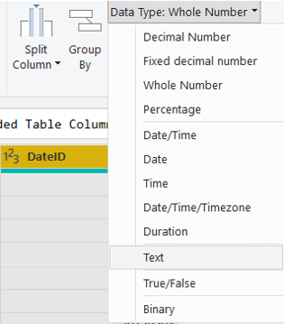
  3. On the top bar, change Data Type to Text
Graphical user interface, application Description automatically generated

  1. Click the Add Column menu
  2. Click Custom Column button
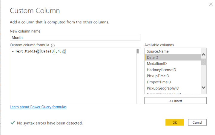
  3. On New Column Name box, set the name as Month
  4. On Custom Column Formula box, set the expression as =Text.Middle([DateID],4,2)
Graphical user interface, text, application Description automatically generated

  1. Click Ok
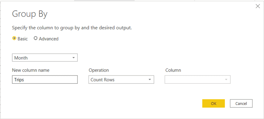
  2. Click the Group By button
  3. Select the Month column
  4. On New Column Name box type Trips
  5. Keep the default Operation, Count Rows
Graphical user interface, application Description automatically generated

  1. Click Ok
  2. Select the Month column
  3. On the top bar, change Data Type to Whole Number
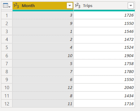
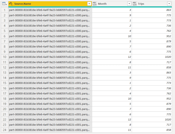
Table Description automatically generated

That’s it, our ETL is ready to be used on the dashboards. Let’s check the execution time of the ETLs

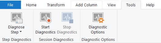
  1. Click Tools menu

Graphical user interface, application, Word Description automatically generated

  1. Click the Start Diagnostics button
  2. Click Home menu
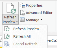
  3. Open the Refresh Preview drop down
  4. Click Refresh All menu item

Graphical user interface, application, Word Description automatically generated

  1. Click Tools menu
  2. Click Stop Diagnostics button

On the left side of the screen, in the query window, you will find a new folder called Diagnostics with two queries inside the folder, holding the results of the diagnostics.

  1. Click the Diagnostics_Aggregate query

Graphical user interface, application Description automatically generated

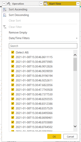
  1. On the StartTime column header, open the drop down
  2. Click the Sort Ascending menu item

Graphical user interface, text, application Description automatically generated

  1. Take note of the time on the first record
  2. On the StartTime column header, open the drop down
  3. Click Clear Sort menu item
  4. On the EndTime column header, open the drop down menu
  5. Click the Sort Descending menu item
  6. Take note of the time on the first record
  7. Calculate the time difference between the first time and the 2nd time you took note

In my example, the total time was 7 seconds. You may find slight differences.

Transformations on Each File

Let’s build the example again, this time building the transformations inside the function, so they would be applied for each file instead of the final result.

  1. Repeat the steps 1-7 from previous steps again
  2. Select the Transform Sample File query
  3. With the Transform Sample File query selected, repeat the steps 9-23
  4. Select the main query, Query1
  5. Remove the last step in Applied Steps window, the Change Type step
  6. Select the first column, Source.Name

Table Description automatically generated

  1. Click the Remove Column button
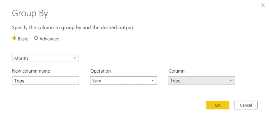
  2. Click Group By button
  3. Select the Month column
  4. In the New Column Name box, type Month
  5. On Operation drop down, select Sum
  6. On Column drop down, select Trips

Graphical user interface, application Description automatically generated

  1. Click Ok
  2. Repeat Steps 24-39

On my example, the execution time results in 4 seconds.

Conclusion

As you may notice, on this example the transformations made on each file performed better than the transformations made after the final combination. This illustrates how important it is to understand this structure and test the performance, deciding which one will perform better for your transformations.

This new feature may not be so obvious, hidden in a Combine button and a complex M code structure, but it’s still much better than possible work arounds for the problem.


The post Power BI reading Parquet from a Data Lake appeared first on Simple Talk.


from Simple Talk https://ift.tt/3bNbT97
via

Monday, January 11, 2021

Oracle archived redo size – the research

In an earlier article, I explained why you might see log file switches taking place much more frequently than expected, with the archived redo files being much smaller than the online redo log files.

When I do presentations about the odd effects that can appear in a fairly ordinary Oracle system, I’m often asked what I did to work out what was happening under the covers. In this article, I will describe a few of the steps I took to investigate this aspect of the logging and archiving mechanism. It’s not rocket science, and most of the time, all I ever do is use methods that have been available for decades.

cpu_count

I started with a review of some default parameter settings and the resulting allocation of public and private redo strands. Somewhere along the line, I pointed out that with “my cpu_count of 48” I got 3 public redo strands.

I don’t actually have a laptop with 48 CPUs – I have a laptop with a single core and 4 CPUs that can do double-threading to look like 8 CPUs, and I was running 19c in a virtual machine configured with 4 CPUs. I set the cpu_count parameter to 48 and restarted the instance – which still told me I had only 4 CPUs until I also set the parameter _disable_cpu_check to true. Now, after startup, I see the following:

SQL> show parameter cpu

CPU count results

Given that I was going to mess with parameters a lot, I switched from a binary spfile to a pure text pfile, (create pfile from spfile command) and ended up issuing the following pair of commands fairly frequently:

shutdown transactional

startup pfile=’./initor19.ora’

That should tell you how I decided that processes defaults to 80 * cpu_count + 40 and found that the manual was slightly wrong in its statement about the default value of sessions (actually 1.5 * processes + 24) but correct in its statement about transactions (1.1 * sessions). I kept restarting the instance after changing the cpu_count in my pfile to see how the other parameters changed.

Redo Strands and In-Memory Undo (IMU)

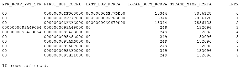
In the previous article, I mentioned the existence of x$ structures but used v$latch_children to find out more about in-memory undo and redo strands. If you want access to the memory for redo strands and in-memory undo, you can query x$kcrfstrand (redo strands) and x$ktifp (in-memory undo) while connected as sys. First, the redo strands:

select
        ptr_kcrf_pvt_strand,
        first_buf_kcrfa,
        last_buf_kcrfa,
        total_bufs_kcrfa,
        strand_size_kcrfa,
        indx
from
        x$kcrfstrand
/

This output shows 3 (= 48/16) public redo strands using 7,856,128 bytes of memory each, and 7 private strands using 132,096 bytes of memory each. The latter was surprising since the number of redo allocation latches told me I should have 644 private strands. Possibly there’s some memory effect that stopped this from happening, or it’s an initial allocation that grows dynamically on demand. Still, I’ve actually been able to disable private redo strands completely by setting an “unlucky” size for the log_buffer parameter which left me with no private strands on startup and resulted in the system activity statistics incrementing the “IMU pool not allocated” and “IMU- failed to get a private strand” statistics on every transaction.

Now the in-memory undo:

select
        ktifpno,
        ktifpxcb                                tx_addr,
        ktifpupb                                undo_start,
        ktifpupc                                undo_cur,
        to_number(ktifpupc,'XXXXXXXXXXXXXXXX') -
                to_number(ktifpupb,'XXXXXXXXXXXXXXXX')  undo_usage,
        ktifprpb                                redo_start,
        ktifprpc                                redo_cur,
        to_number(ktifprpc,'XXXXXXXXXXXXXXXX') -
                to_number(ktifprpb,'XXXXXXXXXXXXXXXX')  redo_usage,
        ktifptxflg
from
        x$ktifp
/

I’ve selected all the rows from this structure (but deleted most of them) to show that Oracle had allocated all 644 even though it had only allocated a few of the private redo strands. If I wanted to query this structure for troubleshooting purposes, I’d probably add the predicate: where tx_addr != hextoraw('00') to limit the output to just the strands currently in use.

The log buffer and the log file

The next step was checking the connection between the log buffer / public strands and the log file. I had set the log_buffer parameter to 60MB with 3 public strands and a log file of 65MB and then made a single process do a lot of work. After seeing the effect on the size of the archived redo log file, I made the initial hypothesis that the three strands had been mapped to 3 areas in the log file. What could I do to confirm this hypothesis?

When I had my 3 strands of 20MB, the first 3 rows of x$kcrfstrand looked like this:

Notice the addresses given in the first_buf_kcrfa and the gaps between them:

  • 0x00000002DE800000 – 0x00000002DD400000 = 0x1400000 = 20971520 (dec) = 20MB
  • 0x00000002DD400000 – 0x00000002DC000000 = 0x1400000 = 20971520 (dec) = 20MB

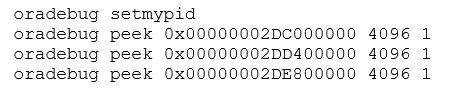
You might assume that the three addresses are the starting addresses of the three memory areas of 20MB each. Take a look at the actual memory content by logging in as a privileged user and executing:

The oradebug peek commands will dump 4,096 (= 8 * 512) bytes starting at the memory location given (note the 0x prefix) to the session trace file and will also echo the first few of those bytes on screen. Here are the first 20 bytes that appeared on screen for the three calls:

A couple of numbers stand out here – the leading 00002201 (but I don’t know what that means) and the 0000025E that repeats down the list, which was the sequence number (v$log.sequence#) of the current online redo log file.

Using the UNIX grep command to find more occurrences of 00000253 in the trace files here are a few lines the first peek command:

from the second peek:

and the third peek:

The left-hand column is the memory address; the next 4 columns hold the 16 bytes starting at that memory address. As you can see, the lines that grep has selected show memory addresses that are separated by 512 (hex 0x200) bytes and the second column is incrementing by one every time. The seco

nd column is the block number within the redo log file where each block of 512 bytes will be written.

There’s an important detail here. The block within file numbers aren’t consistent with blocks that are 20MB apart from each other (the gaps are approximately 0x2000 blocks, i.e. roughly 4MB). This shows that even though Oracle may have allocated three areas of 20MB in the log file, it hasn’t mapped each 20MB of file to a corresponding contiguous 20MB of memory; the mechanisms for using the memory must be a little more sophisticated than that.

To get a finer grained view of the activity, I changed the test to execute a larger number of smaller transactions and then started stepping through a redo strand 512 bytes (one block) at a time dumping 16 bytes at each step. I used a little PL/SQL to write a script to do this:

declare
        n1 number := to_number('&m_head','XXXXXXXXXXXXXXXX');
begin
        for i in 0 .. 127 loop
                dbms_output.put_line(
                                'oradebug peek 0x' ||   
                                to_char(n1 + 512 * i , 'FMXXXXXXXXXXXXXXXX') || 
                                ' 16'
                        );
        end loop;
end;
/

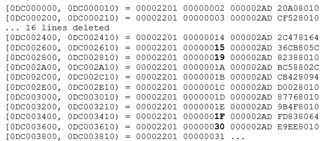
This script produced a list of oradebug peek {address} 16 commands that I spooled to a file then executed from SQL*Plus. You’ll see that I’ve got a substitution variable &m_head that I used to supply the starting address of a redo strand. Here are the results from the start of the first of the three redo strands in the latest test – the 0X2AD in the penultimate column tells you that I’ve switched log files several times since my previous experiments.

You’ll notice that this redo strand starts with blocks 0x2 to 0x15 of the redo file then jumps to block 0x19 and gets as far as block 0x1F before leaving another gap and jumping to block 0x30.

When executing the list of peeks into the second redo strand, you can discover the “missing” blocks:

The result tells us that there’s something very dynamic about how Oracle handles the mapping between the redo log file and the in-memory public redo strands. Even though Oracle seems to use the size of the public redo strands as a sort of “rationing” mechanism, it’s not hard mapping from memory to file. This is good since the log writer would otherwise be making huge jumps around the redo log file to write it every time a session issued a commit. The appearance of large gaps in the lists of block numbers in the previous test must have been something to do with the sizes and numbers of concurrent transactions.

Next Steps

At this point, it’s important to pause for a moment to consider what’s been learned. The experiment established (with a reasonable degree of confidence) that the number of CPUs and the value of the log_buffer parameter have a critical impact on the size and number of the public redo threads and the potential “wastage” of space in the redo log files. You have determined that the actual wastage is then affected by the degree of concurrency of the work going on, and have noted that the pattern of the work (small or large transactions) may make some difference to the way writes to the redo log files are scattered.

The question at this point is – “what do we need to do next?” The answer, I think, is “Nothing”.

So far, what’s been learned provides an argument for picking a suitable size for the redo log files. Any further investigations are probably not going to tell anything useful. This is an excellent moment to stop digging unless you’re seeing some further problem that hasn’t yet been addressed.

On the other hand, there may be some interesting little details waiting to be discovered, and maybe there’s something that might turn out to be useful in a couple of years’ time. Here are a few more thoughts and observations and a few pointers on how to get started – for entertainment value only – that you might think about investigating.

Open Questions

Is the (hypothesized) block number seen in the in-memory redo thread really used to identify the location where that bit of the thread will be written, or is it just a hang-over from a time when the redo writing mechanism was much simpler?

When Oracle writes to the redo log file, does it write sequentially or will it have to jump around the log file? (Is this question answered by the previous one?)

When recovery is taking place, will Oracle read the log file sequentially or will it have to jump around the log file to read redo records in the correct SCN order? (Is this also addressed by the first question?)

Will a single transaction be associated with a single public redo thread until it commits? (If so, how would this affect scalability in the face of a lot of highly concurrent activity?)

One strategy to start finding answers to these questions is simply to dump an archived log file and start comparing the “logical” dump with a raw physical dump.

If you are interested in extending your understanding of the activity as Oracle handles redo, there’s some interesting material in Oracle Core (ISBN 978-1-4302-3955-0). However, for a very detailed examination of the concurrency issues and all the latching that goes on as Oracle moves data between sessions, private redo strands, public redo strands and the log files, Frits Hoogland has spent a lot of time in recent years investigating and writing up the details on his blog. A good starting point would be: https://fritshoogland.wordpress.com/2018/01/29/a-look-into-oracle-redo-part-1-redo-allocation-latches/

Looking at log files

After generating a little over 70 MB of redo by starting three concurrent processes in a loop doing many multi-row updates with commits so that Oracle filled and archived the current log file, I dumped the entire archived log file using the basic command:

alter system dump logfile {archived_log_filename};

Be careful when doing this, the archived log file was just under 65MB, but the trace file was just over 374MB. If you want to see what’s happening with a single transaction, you could limit the log file dump to a single transaction. Modify the update code to report transaction IDs (from v$tranaction.xidusn, xidslot and xidsqn) just before each commit and use one of the transaction triplets in the following command:

alter system dump logfile {archived_log_filename}
xid {xidusn} {xidslot} {xidsqn};

One thing to pick out from the trace file would be an ordered list of “Redo Records”. Here’s how to find their headers with a simple grep command – or an egrep command if you want the “Change Vectors” at the same time:

grep -n "^REDO RECORD" {tracefile_name}
egrep -n -e "^REDO RECORD" -e "^CHANGE" {tracefile_name}

Here are the first few lines of output from my trace file (by this time I was on log file sequence 768 / 0x300)

The thing to pick out is the three-part RBA (redo byte address) which consists of {sequence#.block#.byte#} which tells you exactly where in the file the redo record starts. An interesting bit appeared further down my file:

Take a look at the block numbers: to display these redo records in order (i.e. in SCN order) Oracle is jumping around three different areas of the archived redo log file. It’s important to spot backwards jumps, of course; if all you see are forward jumps, then that may simply be a timing/delay effect.

This result suggests two things: first, recovery does not read a log file sequentially to apply redo at the roll-forward stage; if your system uses multiple redo threads, recovery may be doing far more random I/Os than you had expected. Secondly, when Oracle writes to the redo log file the log writer (or each log writer slave) must be doing something far more complicated than it did in older versions – a writer may be turning a single contiguous piece of log buffer into a number of separate writes corresponding to the different areas of the log file, and that may have to be done with each public strand in turn for a fairly large number of commits.

Of course, it’s just possible (though it seems very unlikely) that with multiple private strands the RBA is no longer an indicator of the truth, maybe RBA 0x000300.0000200d.0014 no longer means the redo record at byte 0x14 of block 0x200d; but you can check that very easily with an O/S block dump. Block 0x200D (8205) will start after 8204 * 512 bytes so a suitable od (octal dump) command would be:

od -j4200960 -N512 -Ad -x {archived_log_filename}

This skips 4,200,960 bytes, prints 512 bytes, gives the address in decimal, and the values in hexadecimal, with the following results for the first 48 bytes of the block:

You’ll spot the 2201, 200d, 300 in the first line here that identify the block and conform to the three (8 byte) values stored at the start of each block in a public strand – so the RBA does mean what it says – and if you look at the whole redo record, you could start matching the contents of the O/S dump with the log file dump:

As a starting point, the first obvious match is the LEN: 0x0780 with the 0780 that appears at the 20th byte, another easy match is the SCN 0x00000b860fc4d7d7 / 0b86 d7d7 0fc4 and SUBSCN 13 / 000d

It looks as if any data in the public strands is copied directly to the log files, and the block address shown in each 512 byte block of memory really is the file block number that the data will be written to. Still, it may take a few more experiments to make us confident that that really is the case.

Conclusion

This article has been an exercise in demonstrating a few tools to poke around inside Oracle to get a broad idea of how some parts of the code are probably working. There hasn’t been much arcane knowledge needed; every tool or mechanism I’ve mentioned has been written about many times in the last 30 years.

In summary, the article:

  • Tweaked a couple of parameters (one of them a hidden parameter)
  • Took advantage of starting Oracle with a pfile instead of an spfile
  • Queried v$latch_children
  • Mentioned v$log.sequence#
  • Queried x$kcrfstrand and x$ktifp – the closest you got to rocket science
  • Used the oradebug peek command
  • Used a couple of grep and egrep commands
  • Looked for patterns in lists of numbers and made a couple of guesses

Then, considering options for further digging, we:

  • Used a couple of “dump logfile” options of the alter system command
  • Used the od command to view the raw contents of a file

What this proved (with some degree of confidence) is why the effective size of the online redo logs (as seen in the archived redo logs) isn’t always the same as the actual size, and how the log writer process and any “recover/replay” mechanism may have to do more work than it used to in earlier versions of Oracle to deal with the multiple public redo strands.


The post Oracle archived redo size – the research appeared first on Simple Talk.


from Simple Talk https://ift.tt/2MUfwQd
via
Visit your parents

Why is it such a cliché to complain about our parents? 

You hear it from friends or in films all the time…”damn, I have to go to my folks for dinner. It’s gonna be rough.” It’s a tale as old as time. 

As our parents age (and retire), they inevitably participate in the world less. They interact with the world far differently than their children, thus often making it more difficult to connect. 

As we age our energy wanes, priorities change, and we have fewer face-to-face interactions in the world. We become content in our comfort zone, playing less offense and opting to hold down the fort. It’s not necessarily bad; it’s just the inertia that bisects the generations. 

Contrarily, as we come-of-age, we tend to go at the world with more fervor. There is more energy to be burned. Life is novel and unexplored. We strive to advance our careers, take risks, and expand our social world. These are beautiful opportunities, but they can also distort priorities and distract us from the people that matter most. The “hamster wheel” is a cliche, but we sure do get stuck on it. It’s the inertia that bisects the generations. 

I get texts from my mom like “what are you watching on tv tonight?” or “did you see the weather report for Thursday?”  My first inclination is to think, “who cares what I’m watching on tv.” But really this is just my mom trying to connect with her son. She’s cracking the door open to go deeper. 

Sometimes when my dad walks by me, he pokes me really hard in the ribs and says “how’s it going, buddy!” This always startles and annoys me so much, but he’s just trying to connect and show affection. 

We have to look for these signals to connect with our parents. They are everywhere. We move thru the world so fast that we miss most of them.

Not everyone is fortunate enough to have a relationship with their parents or have parents that want to connect at all. But there is often an opportunity to bridge that divide, even when it seems impossible to connect.  As our parents age, we can start to do the math on how many more times we will see them. (ex: 2x per year times 15 years. Only 30 more times!) 

It’s key to not miss out on the opportunities to connect. Because as much as small talk can be frustrating, there is gold underneath those basic questions. And looking back, we will be so grateful that we dug a little deeper for it.

Commentary Competition

Enjoyed the topic? Have a relevant anecdote? Disagree with the author? Leave your two cents on this post in the comments below, and our favourite response will win a $50 Amazon gift card. The competition closes two weeks from the date of publication, and the winner will be announced in the next Simple Talk newsletter.

The post Visit your parents appeared first on Simple Talk.


from Simple Talk https://ift.tt/35uFe4l
via
Saturday, January 9, 2021

Kubeflow for data scientists introduction

Kubeflow is a Machine Learning platform that runs on top of Kubernetes and provides end to end functionality for executing machine learning projects. Google created it for internal use of running Tensorflow jobs on Kubernetes, and they later released it as open-source in 2018. Kubeflow has become an essential toolkit for data scientists today since it abstracts them from the underlying complexities of Kubernetes and provides a seamless platform for easy execution and faster delivery of machine learning projects. To appreciate how Kubeflow can make a remarkable difference in a machine learning project, you first need to understand the pain points of data scientists.

Kubeflow for data scientists logo

Why is Kubeflow important for data scientists?

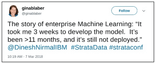
Around four to five years back when the hype of machine learning and data science had just started, everyone tried to capitalize on the trend in a rush. Individuals spent a considerable amount of time and effort to learn machine learning. In contrast, companies pumped millions of dollars overnight to launch their ML and DS projects. Yet, according to a Dec 2019 report, only 22% of companies running machine learning projects could deploy a model to production at all. And more than 43% of the respondents admitted they struggle to scale the ML projects according to the company’s needs.

The main reason behind this high failure rate is that everyone focused only on learning ML and DS concepts with POC work on their local Jupyter notebooks in the initial days. There was no thought process on how to practically execute real-world ML projects and deliver them to production successfully. This lack of understanding became visible when these projects started to fail in companies.

Twitter image about too long to deploy

Since the ML project life cycle differs from the traditional software life cycle, the concept of MLOPs was soon introduced as a framework similar to DevOps to speed up the delivery of ML projects. To bring consistency and ease in the scalable model deployment process, containerization technologies like Docker and Kubernetes were also introduced for ML projects. Kubernetes is an orchestration framework for containers, specifically allowing easier deployment, horizontal scaling, and load balancing for the ML models.

However, as another report suggests, 39% of the data scientists still find it difficult to work with Docker and Kubernetes. This skill gap becomes a challenge for deploying ML models successfully to production. Even though Docker and Kubernetes can make life easy, they are separate technologies and require different expertise than machine learning to make the best use of them.

There was a growing realization that the data scientists should not be exposed to the complexities of managing the infrastructure side of the ML projects and should be given an abstracted platform where they can focus on what they can do best, crunch data, and create ML models. This is where the release of Kubeflow by Google became a game-changer for data scientists, and you’ll see how in the next section.

Features of Kubeflow

As mentioned in the beginning, Kubeflow is an end-to-end platform for creating, training, and deploying ML models and can run on any place where Kubernetes is already present. Kubeflow is now available on Google Cloud Platform, AWS, and Azure as services but you can also install Kubeflow on-premises or your local laptop. Let us now do a deep dive into Kubeflow offerings.

Model building and training

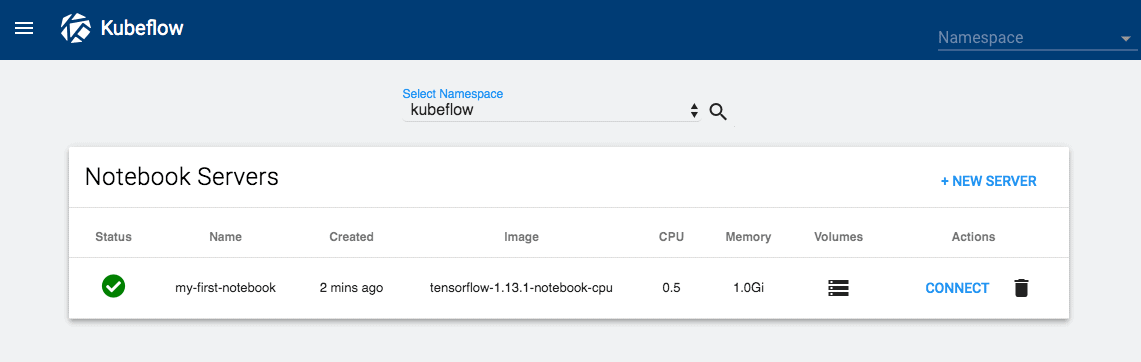
Kubeflow provides managed Jupyter Notebook instances that can be used for experimenting and creating prototypes of the ML models. It supports the popular libraries of Scikit Learn, Tensorflow, PyTorch, XGBoost and you can also carry out distributed training with the help of TF Jobs.

Notebook server Kubeflow for data scientists

Jupyter Notebook on KubeFlow (Source)

Hyperparameter tuning

Finding the right set of hyperparameters for your model is not an easy manual task as it can be very time-consuming and may not even guarantee an optimal set of hyperparameters.

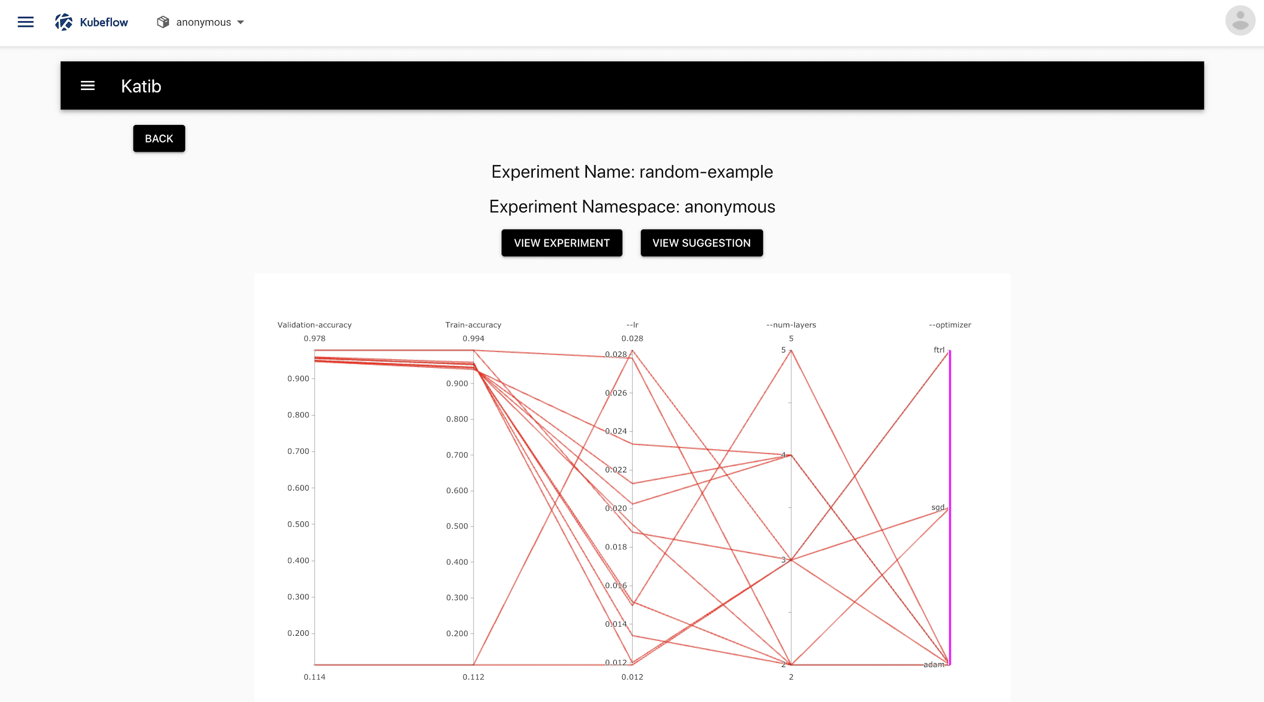
Katib is Kubeflow’s Hyperparameter tuning system that runs on Kubernetes underneath it to automatically optimize hyperparameters for the best results in less time.

Hyperparameter tuning

Hyperparameter Tuning using Kubeflow Katib (Source)

Model deployment and serving

As shown above, deployment and serving of ML models in production in a scalable manner is the most challenging task for data scientists, but Kubeflow has made this task very easy with plenty of serving tools available for your needs

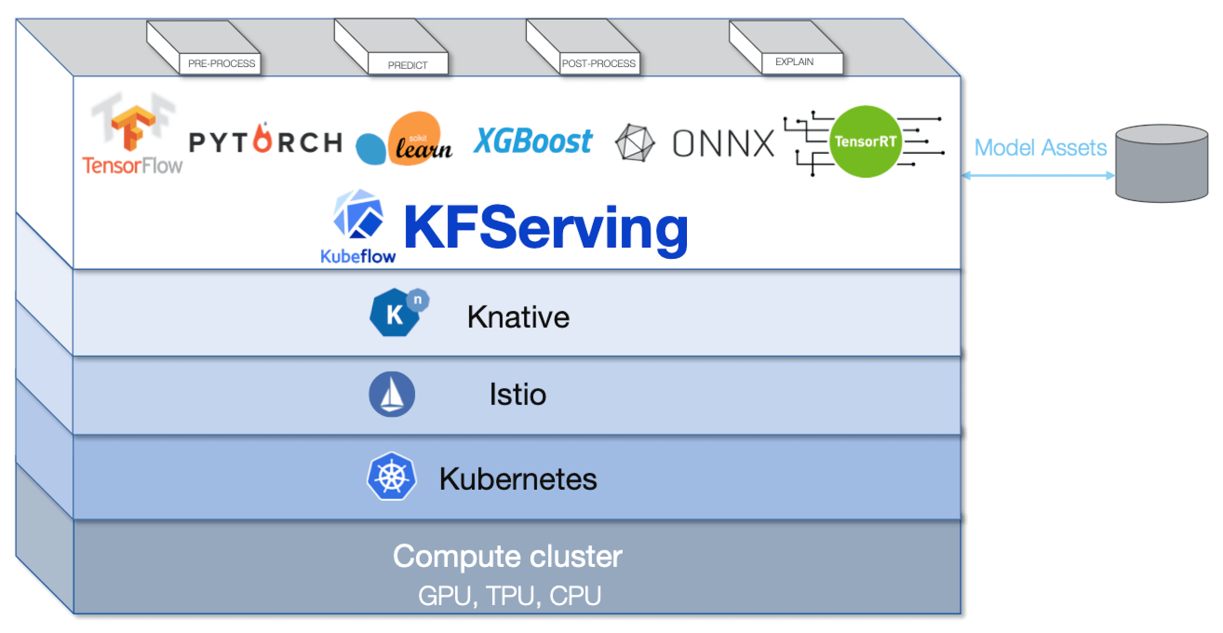
First of all, it provides KFServing which is a model serving tool that supports multiple frameworks like Tensorflow, PyTorch, Scikit Learn, XGBoost, ONNX. Under the hood, KFServing sets up serverless inference on Kubernetes by hiding the underlying complexity from the user. It takes care of autoscaling and health check of the underlying Kubernetes cluster on its own.

Besides, KFServing, there is another option of Seldon Core and BentoML which are other multi-framework supported serving tools. And in case you are working on the TensorFlow model you can also use the TensorFlow Serving that is available on Kubeflow.

KFServing

KFServing (Source)

Portability and flexibility

Even though Kubeflow has various components to cater to different phases of an ML project life cycle, it does not restrict you to use it only for end-to-end purposes. It gives the flexibility to choose one or more components as per your needs, and, to support this flexibility, it also ensures portability across multiple infrastructures and clouds. This enables you to build and train the model externally and then use KubeFlow only for model deployment purposes. Or you may create and train the model on KubeFlow and then deploy it on some cloud for serving.

Cloud platforms

Kubeflow provides portability across clouds and other infrastructure (Source)

KubeFlow pipelines for CI/CD

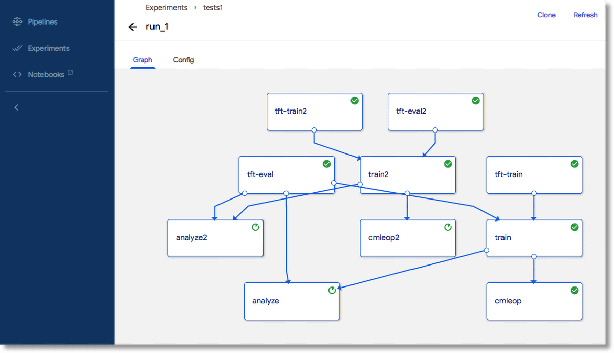
The concept of machine learning pipelines for MLOPs actually comes from the DevOPs pipeline to ensure continuous integration and continuous deployment. Kubeflow CI/CD pipelines not only ensure automation of the ML workflows for faster delivery of changes but are also useful to create workflows that are reproducible for scalability.

Kubeflow pipeline

Kubeflow Pipeline (Source)

Kubeflow Fairing

Kubeflow provides a high-level Python SDK – Fairing for creating, training, and deploying machine learning models locally and more importantly, remotely on Cloud. Fairing abstracts the users from the complexity of working with Cloud by streamlining the training and deployment process with just a few lines of codes so that you can focus only on ML models as data scientists.

As per the current documentation, Fairing supports working with GCP, AWS, Azure, and IBM Cloud.

Example – Kubeflow Fairing with AWS

The example below deals with the House Pricing Prediction problem and shows model creation, training, deployment, and serving using Fairing.

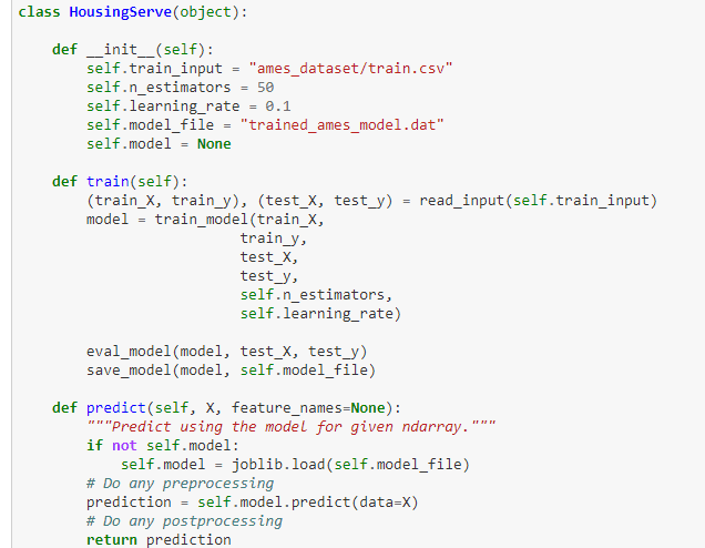
  1. ML Code – This snippet shows the code for training and prediction written inside the HousingServe class. (Additional details are omitted from here to keep the focus on the Fairing part, original code can be found here )

Machine learning code

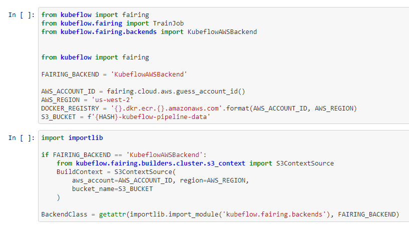
  1. AWS Setup – The next section shows how to set up Kubeflow Fairing with an AWS account, Docker registry, S3 bucket. You will have to replace the details with your AWS details, but the steps remain similar.

  1. Training remotely on AWS – You can submit your ML training job on AWS in just two lines by using TrainJob module of Fairing. The HousingServe class, training data, and AWS docker image are passed as arguments.

  1. Deploy Model on AWS – Similarly, deployment of the ML model on AWS is quite easy with the help of PredictionEndpoint module of Fairing. Make note, this time, you are passing the trained model file in the argument.

  1. Serving Prediction – The earlier step will generate a prediction endpoint which can be used in the following way for serving prediction. Replace the <endpoint> with the output of the above section.

As shown in the example, a Data Scientist only needs to focus on step 1, the ML model creation and other related data pre-processing tasks. All other steps from 2 to 5 are standard Fairing code which is relatively easy to execute for remote training and deployment on the cloud.

Conclusion

This article gave a gentle introduction to Kubeflow for data scientists and touched upon why Kubeflow is an important machine learning toolkit for data scientists. You also saw various functionalities offered by Kubeflow and finally understood Kubeflow Python SDK, Fairing with the help of an example.

If you like this article, you might also like Building Machine Learning Models to Solve Practical Problems – Simple Talk (red-gate.com)

The post Kubeflow for data scientists introduction appeared first on Simple Talk.


from Simple Talk https://ift.tt/3ou3ZVx
via

Wednesday, January 6, 2021

Database version control: Getting started with Flyway

“Database migrations made easy” and “Version control for your database” are a couple of headlines you will find on Flyway’s official website. And let me tell you this, those statements are absolutely correct. Flyway is a multi-platform, cross-database version control tool with over 20 supported databases.
From all my years of experience working as an Architect for monolith and cloud-native apps, Flyway is by far the easiest and best tool on the market to manage database migrations.

Whether you are an experienced data professional or starting to get involved in the world of data, this article is the foundation of a series that will get you through this fantastic journey of database migrations with Flyway.

Background history

Flyway was created by Axel Fontaine in early 2010 at Google Code under the Apache 2.0 license. According to Axel’s words, it all started when he searched for a tool that allows integrating application and database changes easily and simply using plain SQL. To his surprise, that kind of tool didn’t exist, and it makes total sense to me because there were not many options back at that time.

Just to get you in context of what I’m talking about in the previous paragraph, everything we know as DevOps today was conceived around 2009. David Farley and Jez Humble released the recognized “Continuous delivery” book in 2010. Therefore, Axel was, without question, a pioneer in deciding to write his own tool to solve this widespread software development problem: Make database changes part of the software deployment process.

Flyway acceptance was great among the developer community, leading to high-speed growth and evolution. For example, the list of supported databases grew, additional support to multiple operating systems was added, and many more features were included from version to version.

The next step in Flyway’s evolution was Pro and Enterprise editions’ launch back in December 2017, which was a smart decision to secure the project’s progression and viability. Without question, Flyway was already the industry-leading standard for database migrations at that time.

Around mid-2019, Redgate Software acquired Flyway from Axel Fontaine. Redgate’s expertise in the database tooling space opens the door to Flyway for new opportunities in expansion, adoption, and once more evolution!

Database migrations

You are probably already familiar with the term Database migration which can mean several different things within the context of enterprise applications. It could mean to move a database from one platform to another or move a database from a previous version of the DBMS engine to the most recent one. Another common scenario these days is moving a database from an on-premises environment to a cloud IaaS, PaaS solution.

This article is not related to any of these practices mentioned above. This article will get you started with database migrations in the context of schema migrations. Yes, this is another kind of database migration which means the practice of evolving a database schema with incremental, reversible, and consistent changes through a simple approach. This approach enables integrating database changes with version control and application deployment processes.

Before digging deeper into this topic, I would like to address the basic requirements of database migrations. Trust me, this topic is fascinating and full of great information that will help you adopt this practice. Whether you are a software developer, database administrator, or solutions architect, understating database development practices like this is essential to become a better professional.

Evolutionary Database Design is the title of an article published on Martin Fowler’s website in May 2006. It is an extract of the Refactoring databases book by Scott Ambler and Pramod Sadalage, also released in 2006. This lecture goes above and beyond explaining the evolution of database development practices through the years, providing techniques and best practices to embrace database changes in software development projects, especially when adopting agile methodologies.

The approach described in this book sets the stage for a collection of best practices that should be followed to be successful.

DBA and developer collaboration

Software development practices like DevOps demand that people with different skills and backgrounds to collaborate closely, knocking down silos and bottlenecks between multiple teams, like the usual separation between development and operations.

In a database development effort, collaboration is crucial to the success of the project. Developers and DBAs should work in harmony, assessing the impact of the database changes proposed before implementing them. Anybody can take the initiative to start the conversations around whether the database code is optimal, secure, and scalable, or simply to make sure it is following best practices.

Version control

Without question, everybody benefits from using version control. All the artifacts that are part of a software project should be included to keep track of the contributor’s individual changes. Starting from the application code, unit and functional tests, database scripts, and even other code types such as build scripts used to create an environment from scratch, known today as Infrastructure as Code.

All databases changes are migrations

All database changes created during earlier stages of the development phase should be captured, no exception. This approach encourages treating database change files like any other artifact of the application, making sure to save and commit these change files to the same version control repository as the application code to be versioned along together.

Migration scripts should include but are not limited to any modification made to your database schema like DDL (Data definition language) and DML (Data manipulation language) changes or data correction changes implemented to solve a production data problem.

Everybody gets their own instance

It is very common for organizations to have shared database environments. This scenario is often a bad idea due to the imminent risk of project delays caused by unexpected resource contention problems. Or, in other cases, delays are caused by interruptions made by the development team itself. A person working on some database objects modified the objects that were part of a last-minute database schema refactoring.

Everyone learns by experimenting with new things. Having a personal workspace where one can endeavor to explore a creative way to solve a problem is excellent! More importantly, being able to work free of interruptions increase productivity.

Leveraging technologies like Docker containers to create an isolated and personal database development environment/workspace seems like a good way to resolve this issue. Other solutions like Windows Subsystem for Linux (WSL) take this approach to a whole new level, providing an additional operating system on top of the Windows workstation.

Leverage continuous integration

Continuous Integration —CI, for short— is a software development practice that consists of merging all changes from a developer’s workspace copy to a specific software branch.

Best practices recommend that each developer should integrate all changes from their workspace into the version control repository at least once a day.

There is a plethora of tools available to set up a continuous integration process like the one recommended above. The one to choose depends on the size of the organization and budget. The most popular are Jenkins, Circle CI, Travis CI, and GitLab.

According to the theory behind this practice, there are few key characteristics a database migration tool should meet:

  • All migrations must have a unique identifier
  • All migrations must be recorded in a migration history table
  • All migrations should be repeatable and reversible

All these practices and characteristics sound attractive to speed up a database development effort. However, the question is: How and what can we use to approach database migrations easily? Worry no more, Flyway to the rescue!

Flyway logo; database version control

What is Flyway?

Flyway’s official documentation describes the tool as an open-source database migration tool that strongly favors simplicity and convention over configuration designed to facilitate continuous integration processes for any database on any platform.

Migrations can be written in plain SQL, of course, as explained at the beginning of this article. This type of migrations must follow the specific syntax rules of each database engine such as PL/pgSQL for PostgreSQL, T-SQL for SQL Server, PL/SQL for Oracle, etc.

Flyway migrations can also be manually executed through its command-line client or programmatically using the Java API, Docker containers, or Maven and Gradle plugins.

It supports more than twenty database engines by default. Whether the database is hosted on-premises or cloud environment, Flyway would not have a problem connecting by leveraging the included JDBC driver library shipped with the tool.

Flyway folder architecture

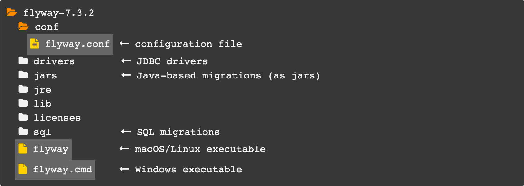
At the time of this writing (December 2020), Flyway’s latest version is 7.3.2. which has the following directory structure:

Flyway folder structure

* Screenshot is taken from Flyway official documentation

As you can see from the folder structure, it is very straightforward; the documentation is so good that it includes a brief description for some of the folders. Let’s take a look in-depth look and define each one of these folders.

The conf folder is the default location where Flyway will look for the database connectivity configuration. Flyway uses the simple key-value pair approach to set and load specific configurations via the flyway.conf file. I will address the configuration file in detail in future articles; for now, I will stick to this simple definition.

Flyway was written in Java, hence the existence of JRE and lib folders. I strongly recommend leaving those folders alone; any modification to the files within these folders will compromise Flyway’s functionality.

The licenses folder contains the teams, community, and third-party license information in the form of a text file; these three files are available for you if you want to take a look and read all details about each type of license.

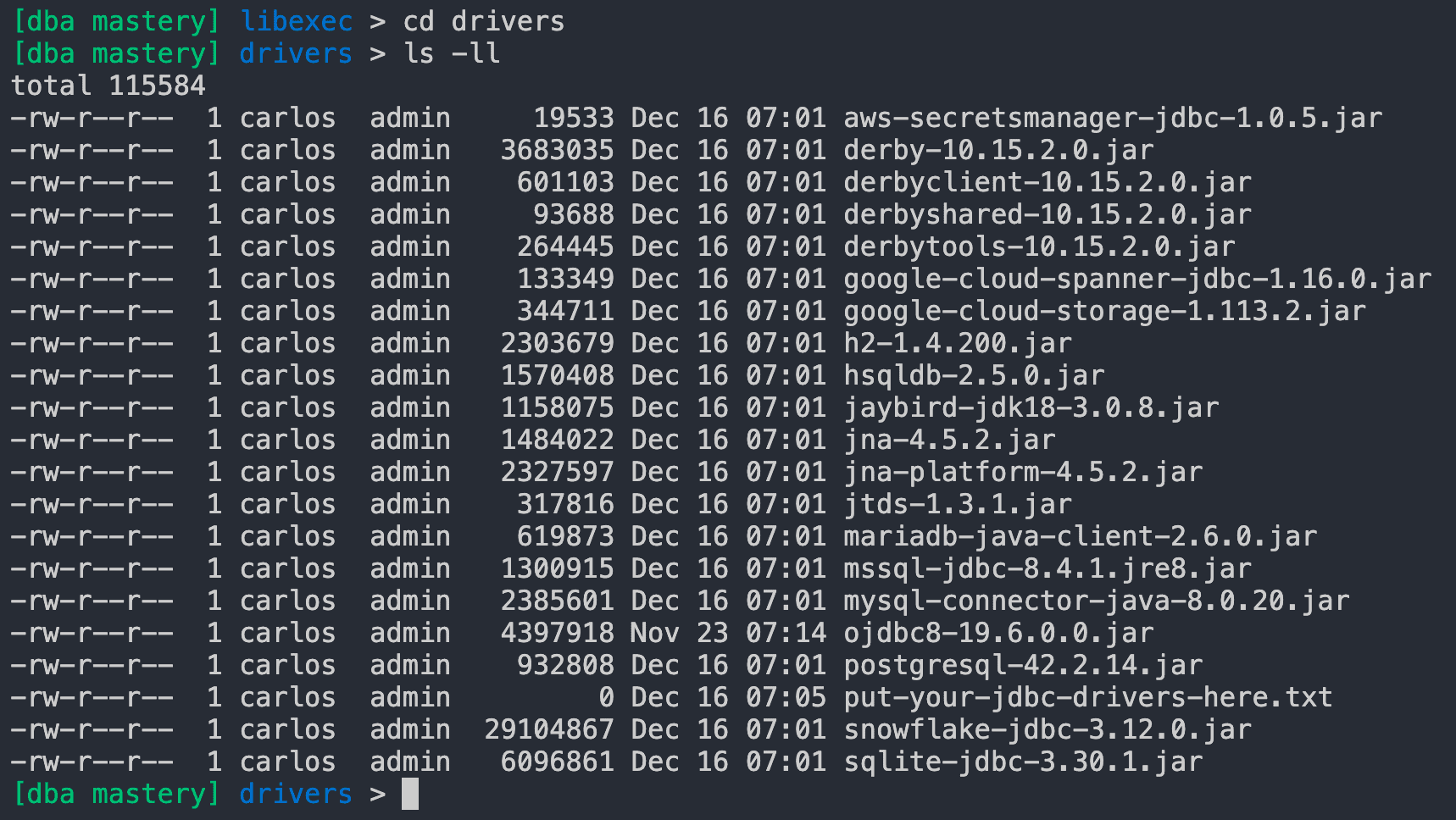
The drivers folder is the place where all the JDBC drivers mentioned before can be found in the form of jar files. I believe this folder is worth to be explored in detail to see what is shipped with the tool in terms of database connectivity through JDBC.

I will use my existing Flyway 7.3.2 environment for macOS. I’ll start by verifying my current Flyway version using the flyway -v command:

Good, as you can see, I’m on the 7.3.2 version. This is the same version used from the official documentation screenshot that describes the folder structure. Now, I will find the actual folder where Flyway is installed using the which flyway Linux command:

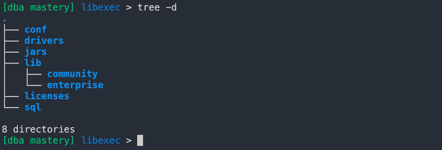
Using the command tree -d, I can list all folders inside the Flyway installation path:

A picture containing graphical user interface, text Description automatically generated

Then I simply have to navigate towards the drivers folder and list all files inside this path using the ls -ll Linux command:

Graphical user interface, text Description automatically generated

Look at that long list of JDBC drivers in the form of jar files; right of the box, you can connect to the most popular database engines like PostgreSQL, Microsoft SQL Server, SQLite, Snowflake, MySQL, Oracle, and more.

Following the folder structure, there are the jars and sql folders where you want to store your Java or SQL-based migrations. Flyway will look at these folders by default to automatically discover filesystem (SQL scripts) or Classpath (Java) migrations. Of course, these default locations can be overridden at execution time via a config file and environment variables.

Finally, there are the executable files. As you can see, there are two types: One for macOS/Linux (Flyway) based systems and one for Windows (Flyway .cmd) systems.

How it works

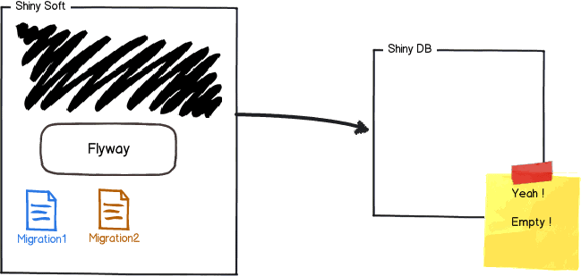
Take a look at the following visual example, where there is an application called Shiny Soft and an empty shell database called Shiny DB. Flyway is installed on the developer’s workstation, where a couple of migrations were created to deploy some database changes.

Diagram Description automatically generated

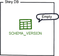
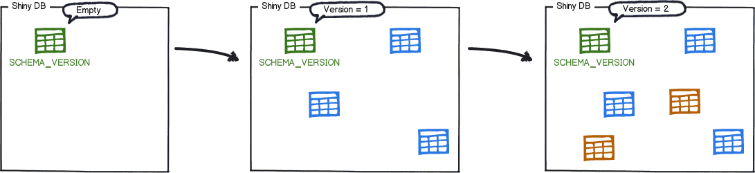
The first thing Flyway will do when starting this project is to check whether the migration history table exists. This example begins the development effort with an empty shell database. Therefore, Flyway will proceed to create the flyway_schema_history table on the target database called Shiny DB.

A picture containing diagram Description automatically generated

Right after creating the migration history table, Flyway will scan and apply all available migrations on its default location (jars / sql)

Graphical user interface, application, Teams Description automatically generated

Simultaneously, the flyway_schema_history was updated with two new records, one for each of the migrations available (Migration 1 and 2).

This table will contain a high level of detail that will help you to understand better how the database schema is evolving. Take a look at the following example:

As you can see, there are two entries. Each has a version, description, type of migration, the script used, and more audit information.

This metadata is valuable and crucial to Flyway functionality. Because it helps Flyway keep track of the actual and future version of your database. And yes, Flyway is also capable of identifying those migrations pending to be applied.

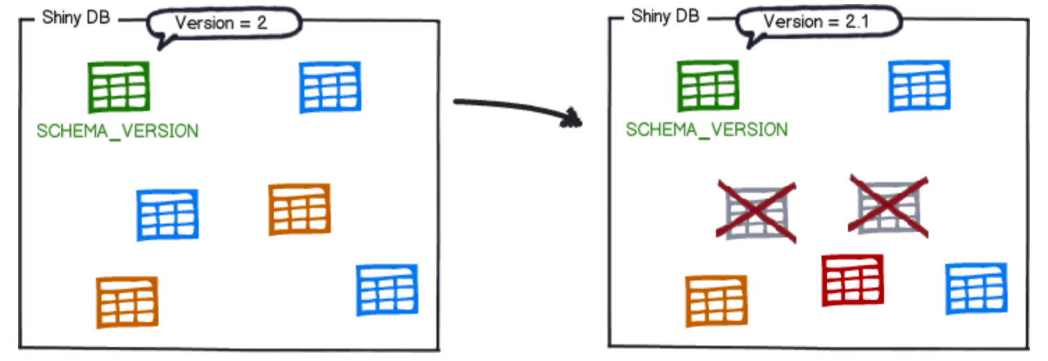
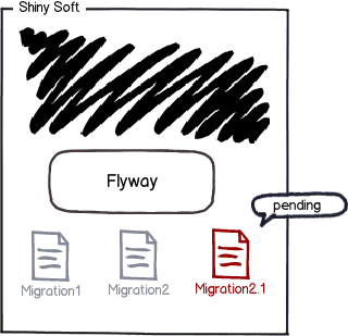
Imagine a scenario where Migration 2 needs to be refactored, creating just one table instead of two. What you want to do is to create a new file called Migration 2.1. This migration will include the DDL instructions to drop the two existing tables and create a new one instead.

Flyway will automatically flag and update this new migration as pending in the flyway_schema_history table; however, it will not apply such migration until you decide to do it.

A picture containing diagram Description automatically generated

Once Migration 2.1 is applied, Flyway will update the flyway_schema_history table with a new record for the latest migration applied: Table Description automatically generated

Notice the third record that corresponds to the database version 2.1 is not a SQL script. Hence the type column record shows JDBC; instead, this was a Java API type migration successfully applied to perform a database refactoring change.

Diagram Description automatically generated

Advantages

At this point, you should be a little bit more familiar with Flyway. I briefly described what it is and how it works. Now, stop to think about what advantages you will get, including Flyway as the central component of your database deployment management.

In software development, as with everything you do in life, the longer you take to close the feedback loop, the worse the results are. Evolving a monolithic legacy database, where any database change is performed following the state-based database deployment approach, could be challenging. However, choosing the right tool for the job should make your transition to a migration-based deployment easier and painless.

Embracing database migrations with Flyway could not be easier. Whether you choose to start with SQL script-based migrations or Java classes, the learning curve is relatively small. You can always rely on Flyway’s documentation to check, learn, and get guidance on every single command and functionality shipped with the tool out of the box.

You don’t have to worry about keeping a detailed control of all changes applied to your database for starters. All the information from past and future migrations are held with great detail in Flyway’s schema history table. This is not just a simple control table. What I like about this schema history table is the level of detail about every single migration applied to the database. You will be able to identify the type of migration (SQL, Java), who, when, and exactly what was changed in your database.

Another major paint point solved by Flyway is the database schema mismatch. This is a widespread and painful problem encountered when working with different environments like development, test, QA, and production. Recreating a database from scratch, at the same time specifying the exact schema version you want to deploy, is a powerful thing. A database migration tool like Flyway will ensure to apply all those changes that belong to a specific version of your application. Database changes should be implanted with application changes.

Conclusion

This article provides a foundation and detailed explanation of Evolutionary database design techniques and practices required to approach database migrations with tools like Flyway.

I also included a summary of Flyway as a database migration tool, starting from the early days, explaining why and how this tool was born. It finally explored its folder structure and components and provided a visual and descriptive example of how this tool approaches database migrations with ease.

Please join me in the next article series, focusing on explaining how to install Flyway’s command-line tool for Linux/macOS and Windows. Also, explore all details related to its configuration through config files and environment variables.


If you liked this, you might also like Introduction to DevOps: Database Delivery

The post Database version control: Getting started with Flyway appeared first on Simple Talk.


from Simple Talk https://ift.tt/3beRcm4
via