Monday, February 22, 2021

A data transformation problem in SQL and Scala: Dovetailing declarative solutions

Part I: Problem Space, SQL Server Simulation and Analysis

This article covers an interesting approach to a software problem. The software to be built must transform data in an operating system file. Would it make sense to include SQL Server in the development environment?

Solving problems first in T-SQL provides result sets against which software results can be compared. Adding to that, query execution plans may serve as blueprints for software development.

In this Part I of the series, I’ll fashion business rules, requirements, and sample data into a denormalized table and query. The query’s WHERE clause includes several logical operators, but its query plan is trivial. To get one that can serve as a software design model, I’ll rewrite the query’s logical connectives as their set operator equivalents. The new query plan is more complex but suggests a logical approach for the software effort.

In Part II, you’ll see T-SQL components realized as structures you know: lists, sets, and maps. What you may not know, though, is how to code algorithms declaratively – e.g. without long-winded loops. The software makes extensive use of map functions, which take functions as arguments and are supported to varying degrees in many Visual Studio languages.

For this article, you’ll need development experience in a relational database and some knowledge of relational theory. For the next, any experience in an imperative or declarative language suffices. Though I’ve written the code in Scala and solely in the functional paradigm, I hope to present just enough background for you to grasp the core strategy of the solutions.

You can download the complete files for both articles. 

Problem Space: Ice Cream

Ice cream manufacturers and retailers, whom I’ll refer to as makers, purvey many flavors. Here are the business rules:

  • There is a many-to-many relationship between makers and flavors.
  • There is a many-to-one relationship from flavor to base flavor (functional dependency: flavor → base flavor).

The term base flavor is an article device not an industry standard.

Participation is mandatory in both. This illustration shows the relationships for five of twelve rows from the operating system file in entity-occurrence style:
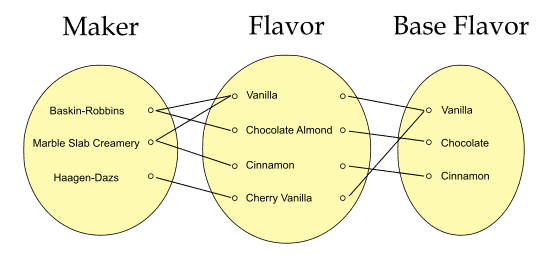
Diagram, venn diagram Description automatically generated

Figure 1. Many-to-many and many-to-one relationships

This is the statement of the data manipulation requirement to be done on the operating system file in software:

For rows in which maker names end in ‘Creamery’ or the base flavor is Vanilla, further restrict these to their flavors being Mint, Coffee, or Vanilla. Return result for all three columns.

The reference to maker name of suffix ‘Creamery’ will result in a non-searchable argument (SARG) that will be handled transparently by the T-SQL but must be addressed directly in the software.

There is a subtle incongruity between the business rules and the data transformation requirement. Do you see it? The file and table will have the same twelve mockup rows but imagine thousands in a real project and how this could impact performance. I’ll point out the issue and resolve it later in a query and take what was learned when developing the software.

Problem Space: The Ice Cream Database

The goal of the table in the simulation database simply is to mirror the data in the file. The many-to-many relationship implies that (Maker, Flavor) is the sole candidate key. Since flavor → base flavor, the table would not be normalized; in fact, it is an intersection table in violation of 2NF. Further, there are no foreign keys or other tables as they would add nothing for the software design.
A picture containing text, black, scoreboard, screenshot Description automatically generated

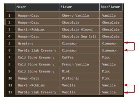
Figure 2. File sample rows having redundancies – not in 2NF

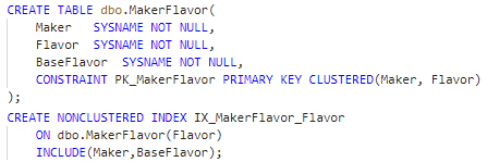
Denormalization is visible in rows 5 and 6 and in 11 and 12. The non-clustered covering index (added post-population) will give a better query execution plan (query plan). More importantly, it will be matched by a key structure in the software – I’m tuning the database only to the extent that it will be relevant later.
Graphical user interface, text, application Description automatically generated

Figure 3. Denormalized intersection table and covering index creation

All database work was done in Azure Data Studio connecting to a local copy of SQL Server 2019. The script is in the download.

Solution Space: T-SQL Queries

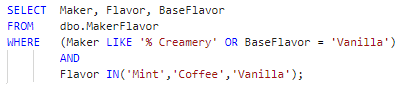
The first goal is to create a result set against which the software result can be verified. Adhering to the business rules and requirements, the query constrains on four logical (Boolean-valued) operators, LIKE, IN, AND, and OR:
Text Description automatically generated with medium confidence

Figure 4. Original query that creates rowset for software verification

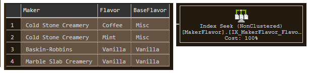
This is the query outcome over the sample rows:
Graphical user interface Description automatically generated with low confidence

Figure 5. Verification rowset with single-step query plan.

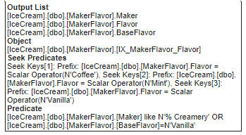
The Index Seek operator over the covering index expands the IN() operator, which implies logical OR, into Seek Keys (for a range scan count of 3), and further constrains on the Predicate as expected:
Text Description automatically generated

Figure 6. Bottom part of expansion for Index Seek operator

All is correct to this point, and I can convert the index into a structure that will be used twice in software. However, the trivial query plan is not as useful as it could be. Relational theory is based on set theory, and the query rewrites next will more directly reflect this. This is important because the transformation algorithms in the software will all be set-based.

Query Rewrite I

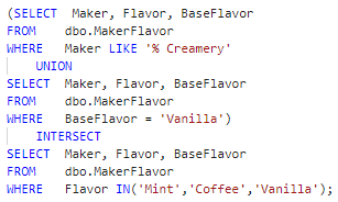
The second goal, as you recall, is to fashion a query whose query plan will serve as a model for the software design. The trick I’ll employ is to replace the logical connectives OR and AND with their T-SQL equivalent set operators UNION and INTERSECT.
Text Description automatically generated

Figure 7. Query rewrite using set-based operators

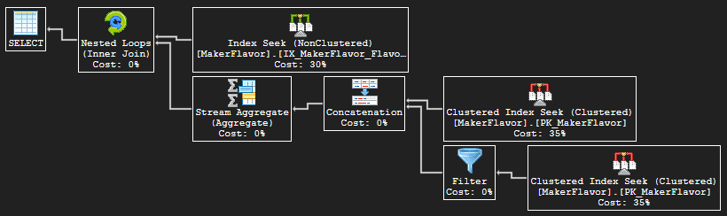
It produces the detailed query plan I’m looking for:
A screenshot of a computer Description automatically generated with medium confidence

Figure 8. Query plan for Figure 7

The outer input uses the same non-clustered covering index and Seek Keys for range scans (scan count remains 3) as the original query but without the Predicate. Instead, each outer row directly joins via Nested Loops (Inner Join) on all columns to the rowset produced by the union of the Creamery and base flavor rows (discussed next). The Nested Loops operator, then, accomplishes a row-by-row set intersection.

In the inner input to Nested Loops, the upper Clustered Index Seek on the primary key is for the LIKE(% Creamery) condition. Although the value to the LIKE logical operator is a non-SARG, a true index seek range scan (not table scan) is done on each outer row’s (Maker, Flavor) prefix, during which the LIKE Predicate can be applied. The lower Clustered Index Seek parallels the upper, differing only in the predicate condition: BaseFlavor = N‘Vanilla.’ Since the Inner Join is done on the superkey – i.e. all columns – and since flavor → base flavor, either lower input branch can produce at most one row. If both produce a row, they must, therefore, be the same row.

The Concatenation simply appends one output to the other – think UNION ALL in T-SQL. To get the T-SQL UNION, then, the Stream Aggregate (Aggregate) operator collapses duplicates via grouping (and no aggregate expressions are computed). Specifically, both Concatenation and Stream Aggregate show only the same Output List, which consists of column header Union 1004, Union 1005, and Union 1006, and their rows are returned to the query.

This query plan lends all the information needed to create index simulators and filter and map operations and algorithms in the software. An optimization, though, remains unaddressed – so almost all.

Query Rewrite II

There is no index on the BaseFlavor column, but in the middle subquery from Figure 7 above, BaseFlavor is constrained on value ‘Vanilla.’ This suggests that the lower-level software might need a data structure(s) and algorithm(s) to support the restriction. To start the analysis, I’ll create this covering index, which parallels that on the Flavor column:

Text Description automatically generated

Figure 9. Covering index on BaseFlavor key

The proposed index has no effect on the query plan in Figure 8 above, nor the original query plan in Figure 5. This is not proof, though, that separate resources are not needed in software to enforce the restriction.

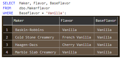
The next illustration shows the subquery run in isolation. A minor point is that the Query Optimizer chooses an Index Seek on the new index in place of an Index Scan using IX_MakerFlavor_Flavor. The central point is that subqueries that form part of a larger, single-statement T-SQL query will be translated into individual software resources that can and will be accessed in isolation.
A screenshot of a computer Description automatically generated with medium confidence

Figure 10. Query in lower half of UNION run in isolation

Now rerun the query but this time constrain the ‘Vanilla’ value by the Flavor column:
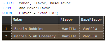
Table Description automatically generated

Figure 11. Constraining on Flavor column yields two fewer rows

This is not an idle thought experiment. The former result set contains two extraneous rows – column Flavor values being ‘French Vanilla’ and ‘Cherry Vanilla’ – that are not in the result set from Figure 4. The software effort needs a decision as to which constraint to enforce. Whether in queries or software transformations, performance is better served when rows not needed are culled early. The question I posed early on regarding the mismatch between the business rules and requirement can now be restated: Can the restriction on BaseFlavor be replaced by that on Flavor and still be correct?

Constraining on the one side of a many-to-one relationship as does the top query form (BaseFlavor) is not wrong per se but is the root of the performance issue here. A business rule, however, signals the solution. The second states flavor → base flavor. Given this, and since the query’s set intersection operation removes rows not matching on the Flavor column, the T-SQL can constrain on the many side (Flavor) without affecting correctness. The implication for software is that it obviates the need for special structures – those for simulating the proposed index to start the section – and handling (algorithms), as will be made clear in Part II.
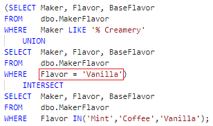
Text Description automatically generated

Figure 12. Query in final form

Testing: A Note on the Sample Data

Say set A denotes the rows produced by the query that restricts on the three flavor names and set B the rows from the union of the two other queries. Given the sample data, it happens that A B and hence B ∩ A = A. Therefore, the query on flavor names alone yields the same result as the full query and the knowledge of which can aid testing.

It is important to realize that this outcome is entirely data-dependent. The proper subset relationship may not hold over an operating system file having different data, and the software will make no assumptions regarding this limited analysis. In general, it is never a good idea to deduce business rules from data that can change over time. With that caveat in mind, sample runs done here and in software over these rows can only boost confidence in results.

In Conclusion

You saw how business rules and software requirement were mapped to a single intersection relational table in which normalization and referential integrity were nonessential. The initial query on the table provided the rowset against which the software result could be verified, but its query plan was inadequate as a pattern from which the software design could proceed.

Rewrites using T-SQL set operators did yield a query plan as software blueprint and provided other insights as well, chief among them the optimization of the base flavor column.

Last Word

Neither loops nor branches were used in any of the T-SQL work, but that doesn’t mean they aren’t there. They are – visible underneath in the query plans, which describe the process steps (operators and data flow) the SQL Server database engine follows to produce results. A salient example of looping is the Nested Loops operator used in the T-SQL rewrite query plan to match each outer row to an inner row, i.e. perform the INTERSECT. This style of coding, in which the logic of the computation is expressed rather than the lower-level control flow detail, is declarative programming, and is a major theme of this series. (The latter being imperative programming.)

The next article, which uses functional programming to solve the series’ problem, continues in this vein. The logic written to the map and filter functions encapsulated in the data structures is again compact and elegant, even as the compiler translates it to control flow statements.

Translating insights gained here into functional programming will be straightforward but not paint-by-numbers simple. You may have found this discussion challenging – I hope stimulating – and may find Part II the same as well.


The post A data transformation problem in SQL and Scala: Dovetailing declarative solutions appeared first on Simple Talk.


from Simple Talk https://ift.tt/2OXzYAB
via

SQL Server authentication methods, logins, and database users

Setting up and managing SQL Server security is an important part of building and maintaining your SQL Server environment. SQL Server security is a vast topic that cannot be covered in a single article. This article starts with a few foundation topics of SQL Server security: SQL Server Authentication methods, logins and database users.

Authentication methods supported

There are two different authentication methods for connecting to SQL Server: Windows and SQL Server.

Windows authentication requires a user to first authenticate to Windows with their login and password. Once a user has been authenticated to Windows, they can then connect to SQL Server using Windows authentication. That is, provided their Windows account has been granted access to SQL Server via a login (more on logins later). Windows authentication is tightly coupled with Windows Security and is also known as Integrated Security. Windows authentication works great when a person is part of a Windows domain.
But there are times when people can’t connect to Windows; this is where SQL authentication comes in. SQL Authentication is less secure than Windows Authentication. In order to connect to SQL Server using SQL authentication, a person needs to provide a login and password when they connect. The password for a SQL Authenticated login is stored in the master database. Because the password is stored in a SQL database, it is more easily hacked. It can also be backed up and restored with a database backup which is why it is less secure than using Windows authentication.

Windows Authentication is the default authentication mode when installing a SQL Server instance. In order to support SQL authentication, you need to configure SQL Server to support mixed mode authentication. When mixed mode is used, both Windows and SQL authentication can be used to connect to SQL Server. If SQL Server is not set up to support mixed mode, then only Windows accounts can connect to SQL Server.

Because SQL authentication is less secure than Windows Authentication, it is recommended that you only set up your SQL Server instance to support mixed mode if you have a requirement to support users or applications that can’t connect to Windows. Even though Windows Authentication is more secure and the recommended practice for connecting to SQL Server, many custom application software vendors still don’t support connecting via Windows authentication.
Setting up SQL Server to support different authentication modes

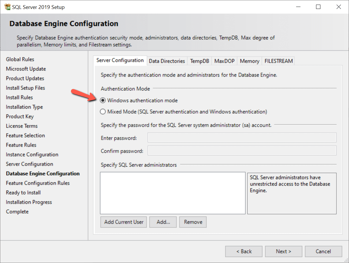
When installing SQL Server, you have the choice to support only Windows authentication or both authentication methods, which is known as mixed mode. During the installation process, you decide whether or not to use mixed mode when defining the database engine configuration, as shown in Figure 1.

Figure 1: Selecting Authentication Methods

Windows Authentication is selected as the default shown with the red arrow in Figure 1. If you need to support both Windows and SQL Server authentication, then you would select the “Mixed Mode” radio button. Upon clicking this button, the SA account password boxes would become enabled, and you would need to specify a password for the SA account. When only Windows authentication is selected, the SA account is disabled. To secure the SA account when you are using mixed mode you can disable the SA account after it is enabled.

How to determine which authentication methods are supported

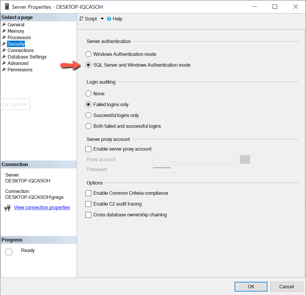
You can check to see which authentication method is configured in several ways. One of those ways is to use SQL Server Management Studio (SSMS). To use SSMS, first right click on the Instance name and select the Properties option. When I do that on my instance, the properties page in Figure 2 is displayed.

Figure 2: Determining Authentication Mode

Figure 2 shows that my instance supports mixed mode authentication because the radio button next to the red arrow is enabled.

Another method to check which authentication modes are set up is to use TSQL code. The code in Listing 1 displays the Authentication mode setup.

SELECT CASE SERVERPROPERTY('IsIntegratedSecurityOnly')   
          WHEN 1 THEN 'Windows Authentication Only'   
          WHEN 0 THEN 'Windows and SQL Server Authentication'  
       END as [Authentication Mode];

Listing 1: Displaying Authentication mode

Changing authentication methods After SQL Server is installed

There are times when you might want to change the authentication settings for a SQL Server instance. This might occur if you used the default settings during installation to support Windows authentication only and later acquired some software that can only connect using SQL Server authentication. Or possibly you want to make your instance more secure by removing support for SQL Server authentication. The authentication options can be easily changed using the properties page in SSMS shown in Figure 2.

If I wanted to change my instances to support only Windows authentication, all I would need to do is click on the “Windows authentication mode” button in Figure 2, and then click on the “OK” button to apply that change. After making this property change, I would need to restart my instance for this change to take effect.

SQL Server logins

In order to connect to SQL Server, one must have access to SQL Server. Access is granted via a login. A login is also known as a security principal, and is stored in the master database. There is one exception, and that is accessing a contained database. With contained databases users connect directly to database without the need for a login in the master database. More on contained databases in future articles.
There are three types of logins that are stored in the master database: Windows user, Windows group, and SQL. Let’s review each of these different types of logins.

A Windows user login provides access for a single Windows user. When creating this type of login, no password is needed when defining the login in SQL Server. This type of login requires the user to first validate their login by logging into the Windows domain. The Windows domain stores the password.

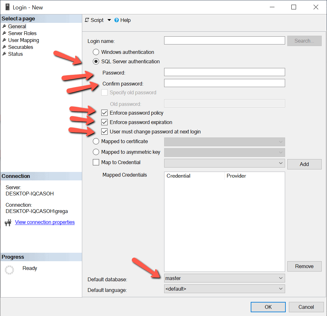
A SQL Server login is similar to a Windows login in that it provides access to SQL Server for a single user, but it is different than a Windows login because the password for a SQL login is stored in the master database. Therefore, when setting up a SQL Server login, a password needs to be provided for the login along with a few other password options, as shown in Figure 3.

Figure 3: Setting up a SQL Server Authenticated Login

Figure 3 shows that a SQL Server Login can be enabled to enforce Windows password policies and expiration and can require a user to change the password upon their first login. Microsoft added these new password features when SQL Server 2005 was released. For applications to support these new password features, they can use the NetValidatePasswordPolicy API.

The last type of login, a Windows group login, is similar to a Windows login but slightly different. A Windows group login provides access to a SQL Server instance for every Windows login that is a member of the group. Windows groups are a great way to provide access to many Windows logins with only having to define a single login in SQL Server. Using a Windows group, access to the SQL Server instance can be maintained by adding or removing group members. Using Windows groups helps minimize security management efforts and troubleshooting login related security issues.

If you look at the bottom of the screenshot in Figure 3, you will notice a “Default Database” setting for a login. The default database setting when creating a login is the “master” database. When setting up a login, the default database can be changed to any database on the server. Best practice is to set the default database to a database that the user will use when connecting to SQL Server.

Windows logins are considered more secure because of the way the password for the login is stored. The password for a Windows login is stored using true encryption. Where as the password for a SQL Login is not encrypted, instead it is hashed. Because a SQL login is hashed makes it easier to crack the password. Windows logins also require domain admin’s to set up the login and password, where as SQL logins the database administrators set up the login and password. By having the domain admin’s managing login passwords provides another layer of security, commonly called separation of duties. By separating the duties of creating and managing Windows logins from managing databases and access to databases, provides an additional security controls to gain access to data stored in SQL Server.

Creating a login to SQL Server allows users to connect to SQL Server. But a login alone doesn’t provide users access to any data in the different databases on the server. For a login to read and/or write data to a database, the login will need access to one or more databases. A login can be set up to have access to many databases on an instance if required.

Database users

A database user is not the same as a login. A login provides to a user or application the ability to connect to a SQL Server instance, whereas a database user provides the login rights to access a database. Each database a login needs access to will require a database user to be defined, except when a login has been given sysadmin rights. When a login has sysadmin rights, they have access to all database, without being mapped to a database user. This association between a login and a database user is known as a user mapping. User mappings for a login can be created during login creation or later for logins that have already been set up.

Creating a database user while creating a new login

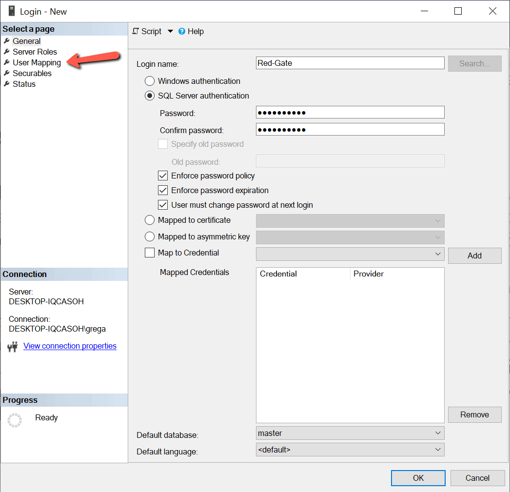
To show how to provide user mapping when a new login is created, I will create a new SQL Server login named “Red-Gate”. The screenshot shown in Figure 4 shows the “Login – new” window where I will define this new login. To bring up this window, I expand the “Security” tab under my instance, and then right-click on the “Logins” option and then select the “New Login…” item from the drop-down.

SQL Server authentication methods

Figure 4: Creating Red-Gate Login

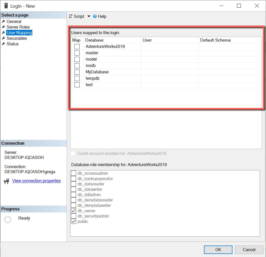
In figure 4, I enter “Red-Gate” for the login name and entered the password for this SQL login in the dialog boxes provided. To provide database access for this new login, I click on the “User Mapping” option in the left pane. When I do this, the window in Figure 5 is displayed.

Figure 5: User Mapping Window

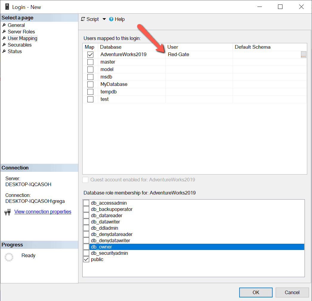
A red box shows the list of databases in Figure 5, where my new login can be mapped. In order to map my “Red-Gate” login to the “AdventureWorks2019” database, I would just need to click on the “Map” checkbox next to the AdventureWorks2019 database. When I do that, the screenshot in Figure 6 is displayed.

Figure 6: Mapping Login to database

After checking the Map box, the name “Red-Gate” is automatically populated in the “User” column for the AdventureWorks2019 database. This interface automatically generates a database user name the same as the login to which it is mapped. Database user names don’t need to be the same as the login. If I wanted my database user name to be different, I could just type over the “Red-Gate” name and specify whatever database user name I wanted. Mapping a login to a database users only provides that login access to the database, but it doesn’t give the login access to read or update data in the database. In future articles I will be discussing how to provide read/write access to database objects.

Suppose I wanted to map my new “Red-Gate” login to additional user databases. In that case, I could do that by just checking on another “Map” checkbox next to the additional databases. For this example, I only want to map my new “Red-Gate” login to the “AdventureWorks2019” database. To finish up mapping my “Red-Gate” login to the “Red-Gate” database user I just need to click on the “OK” button.

Creating a new database user and mapping it to an existing login

There are times when a login has already been created, and it just needs access to one more database. For example, suppose I now wanted my established Red-Gate SQL Server login to access the database named “MyDatabase”. To give the Red-Gate login additional database access, I have a number of options. One option would be to just modify the user mappings by changing the properties on the login. This would be similar to how I just added the user mapping when I created the Red-Gate login.

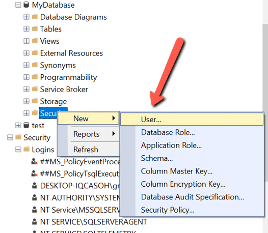
Another option is to add a new database user to the “MyDatabase” and then mapping that new database user to the Red-Gate login. To create a new user in the database “MyDatabases” I would first expand the database, right-click on the “Security” item, hover over the “New” item, and then click on the “User…” item, as shown in Figure 7.

Figure 7: Bring up the new database user dialog

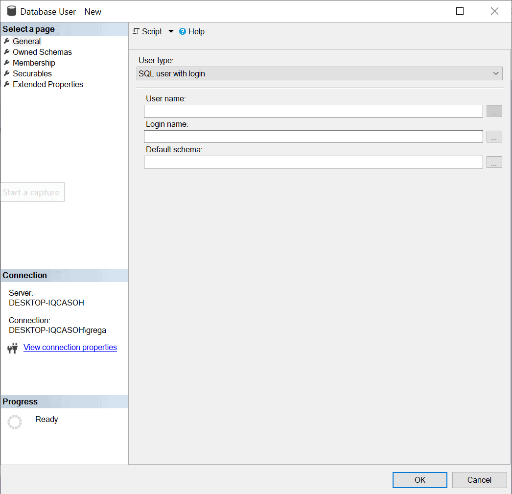
When I click on the new “User…” menu item, the window in Figure 8 is displayed.

Figure 8: Adding a new database user

To give the Red-Gate login access to MyDatabase, I need to fill out the form in Figure 8. The first item in Figure 8 to consider is the “User Type”. This field defaulted to “SQL User with Login”. There are four other types: SQL user without login, User mapped to a certificate, User mapped to an asymmetric key, and Window users. Since I am creating a database user that will be mapped to a SQL login, I use the default. Next, I enter the database user name for the user I am creating. It could be any name, but I prefer to make the database user name match the same name as the login it is associated with. Therefore I enter “Red-Gate” in the “User Name” field. I next map my new users to a login. To do the mapping, I can either type in “Red-Gate” for the login or use the ellipsis button (…) to browse through the list of logins already created and select one.

The last item needed is to define a default schema for this login. A schema name is associated with a database object collection owned by a database user. By default, each database has a schema named “dbo” owned by the “dbo” user account. You don’t need to specify a schema when you define a new database user. If one is not specified when defining the database user, the “dbo” schema will be the default schema. Since this article is just a primer, I will discuss the different aspects of schemas. I’ll leave that for another article. When I create my new Red-Gate database user, I’ll leave the default schema item empty and let the create new users process set the default schema automatically to “dbo”.

Once I’ve created my new user, I can verify it exists in the database by expanding the “User” item under the “Security” folder in Object Explorer. You can also create a new database user and map it to a login using a script. Listing 2 is an example of using TSQL to create the same login I just created using the point and click method.

USE [MyDatabase]
GO
CREATE USER [Red-Gate] FOR LOGIN [Red-Gate]
GO

Listing 2: Create a Red-Gate database user using a TSQL script

SQL Server authentication methods, logins, and database users

To connect to SQL Server, a person or process needs to authenticate. There are two different methods to authenticate to SQL Server: Windows and SQL Server. Windows is the more secure and recommended method for connecting to SQL Server. Each connection that authentications to SQL Server gains access to the instance via a login. Logins are defined at the server level. Logins by themselves don’t provide access to data within SQL Server. To gain access to data in a database, a login needs to be mapped to a database user. The authentication methods, logins, and databases users provide the basic security foundations for SQL Server security.

If you liked this article, you might also like Understanding SQL Server Recovery Models.

The post SQL Server authentication methods, logins, and database users appeared first on Simple Talk.


from Simple Talk https://ift.tt/3aI58Ev
via

Creating Reports using Oracle SQL Commands

Reports are widely used by managers, analysts etc., to do data analysis and make business decisions. Report developers mostly use different reporting tools that are available in the market.  As most of the reporting tools are not open sourced, it is difficult to provide access to tools. You can download the code here.

Analysts can now create reports using Oracle SQL and SQL*Plus commands, SQL*Plus commands help facilitate output formatting which gives users better readability at data. 

Difference between GROUP BY and BREAK/COMPUTE Commands? 

GROUP BY command is a SQL command which returns only summary information, this command is one of the most used command on day-to-day basis. 

BREAK and COMPUTE are SQL*Plus commands, we use break and compute commands when we need detail (individual) along with summary information 

BREAK and COMPUTE Commands: 

Compute command lists the desired summary information at one or more break points. Break command defines break points. We can use break command without a compute command, but we can’t use a compute command without break command.  

In this article, I will provide a set of examples to showcase how to create reports using SQL 

Getting Started: 

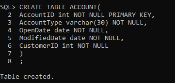
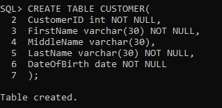
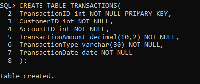
In order to follow the below examples, you will need to create three tables Account, Customer and Transactions by executing below code in Oracle 

Account Table: 


Customer Table: 


Transaction Table: 


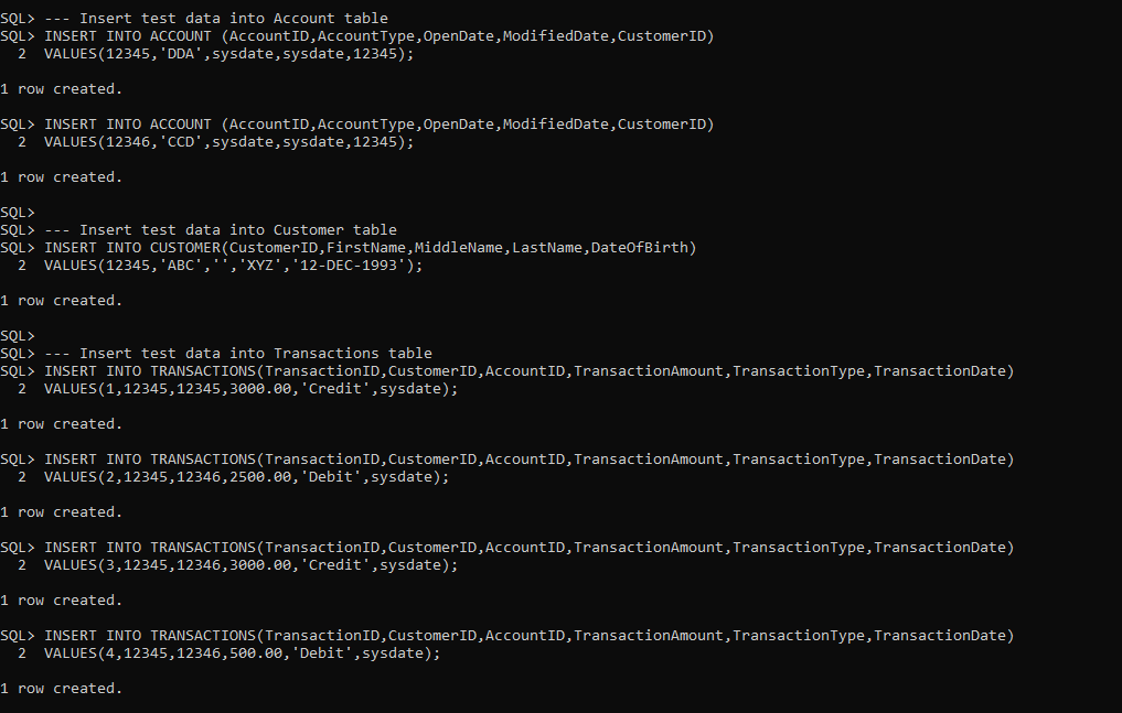
INSERT Test Data: 


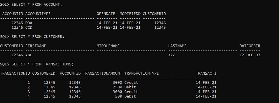
After executing the above SQL code, we will be able to see that records have been inserted into Source tables as shown in below image 


Break and Compute Commands Syntax: 

break on {expression|column_name|row|page|report} [skip n|skip page] [duplicate|noduplicate] 

compute function of column_name on break_point 

We can give only one break command but multiple break points within that command. 

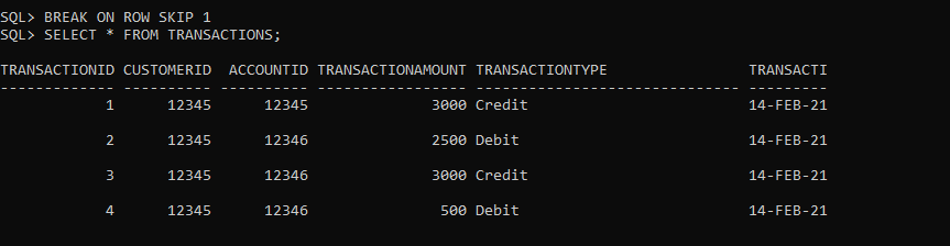
Display rows with blank lines between rows: 

Break on row skip 1 

Select * from Transactions;   


Creating a Report: 

Add Page Headers and Footers: 

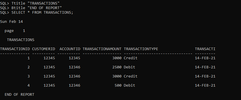
We can add page headers and footers using Ttitle (top title) and Btitle (bottom title) are top and bottom title 

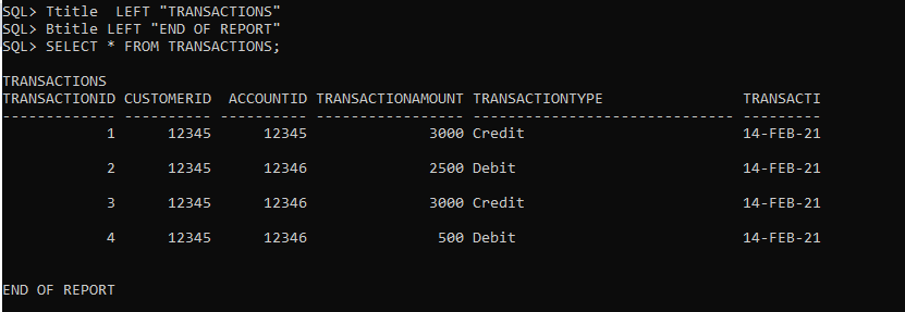
Location of the titles can be defined using “left”, “right”, “center” keywords. 

Ttitle “TRANSACTIONS” 

BTitle “END OF REPORT” 

SELECT * FROM TRANSACTIONS; 


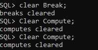
Clearing Break, Compute Commands: 

Clear Break 

Clear Compute 


Clearing Specific Column Command: 

Column ColName clear — to clear a specific column 

Clear Column — to clear all columns 


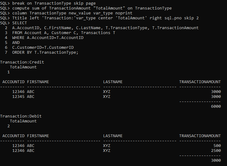
Report: 

Set feedback off 

Clear Break 

Clear Compute 

Clear Columns 

break on TransactionType skip page 

compute sum of TransactionAmount "TotalAmount" on TransactionType 

column TransactionType new_value var_type noprint 

Ttitle left 'Transaction:'var_type center 'TotalAmount' right sql.pno skip2 

SELECT  

A.AccountID, C.FirstName, C.LastName, T.TransactionType,  T.TransactionAmount 

FROM Account A, Customer C, Transactions T 

WHERE A.AccountID=T.AccountID 

AND 

C.CustomerID=T.CustomerID 

ORDER BY T.TransactionType; 


Summary:

As shown in the above example we can create reports using SQL. Analysts or Developers can use this approach during data analysis or to work on a production issue on an adhoc basis


The post Creating Reports using Oracle SQL Commands appeared first on Simple Talk.


from Simple Talk https://ift.tt/2ZDZ8GD
via

Thursday, February 18, 2021

Function (and SQL Prompt Snippet) To Get Next Date By Day Name/Offset

As I have been building my Twitter management software, I have been doing a lot more ad-hoc, repetitive coding using T-SQL directly. When I was generating new tweets for upcoming days, a bit of the process that got old quick was getting the date for an upcoming day (the primary key for my tweet table is the date, the type of the tweet, and a sequence number). After having to pick the date of next Tuesday… I had to write some more code (because a true programmer doesn’t do repetitive work when code can be written… even if sometimes the code doesn’t save you time for days or weeks.

So this following function was born from that need, and it is something I could imagine most anyone using semi-regularly, especially when testing software. This is the code (with a bit of reformatting):

NOTE: The code is available in my Github repository for my database design book here: dbdesignbook6/Useful Code at master · drsqlgithub/dbdesignbook6 in the Tools Schema.sql file. 

CREATE OR ALTER FUNCTION Tools.Date$GetNthDay
(
     --Spelled out the name of the day of the week
        @DayName varchar(20), 
     --positive or negative offset from the current week
        @NumberOfWeeks int = 0, 
        @DateValue date = NULL --the day to start the calculation
)
RETURNS date
AS
 BEGIN 
    --if the date parameter is NULL, use current date
    SET @dateValue = COALESCE(@DateValue,SYSDATETIME());

    --this is a stand in for a calendar table to make it portable and not subject
    --to any date settings
    DECLARE @DaysOfWeek table (DayNumber int NOT NULL, 
                               DayName varchar(20) NOT NULL);

    --load 14 days to make the math of days between days easy
    INSERT INTO @DaysOfWeek(DayNumber, DayName)
    VALUES(1,'Sunday'),(2,'Monday'),(3,'Tuesday'),
           (4,'Wednesday'), (5,'Thursday'),(6,'Friday'),
           (7,'Saturday'), (8,'Sunday'),(9,'Monday'),
           (10,'Tuesday'),(11,'Wednesday'), (12,'Thursday'),
           (13,'Friday'),(14,'Saturday');

     --get the day number of the date that was passed in 
     --on the DateValue parameter
     DECLARE @CurrentDayNumber int = (SELECT MIN(DayNumber) 
                                      FROM @DaysOfWeek 
                                      WHERE DayName = DATENAME(weekday, @DateValue));  

      --get the next day number in the table to get the number 
      --of days to add
      DECLARE @NextDayNumber int = (SELECT MIN(DayNumber) 
                                    FROM @DaysOfWeek 
                                    WHERE DayName = @DayName 
                                      AND DayNumber >= @CurrentDayNumber); 

     --add the number of weeks to the date you calculate to be 
     --the upcoming day that matched your parameters
      RETURN (DATEADD(WEEK,@NumberOfWeeks,
               DATEADD(DAY, @NextDayNumber – @CurrentDayNumber, @DateValue)));
 END;
GO

To see the code in work, Here are a few examples:

SELECT Tools.Date$GetNthDay ('Tuesday', 0, '2021-02-17');

Returns: 2021-02-23

SELECT Tools.Date$GetNthDay ('Tuesday', 1, '2021-02-17');

Returns 2021-03-02

SELECT Tools.Date$GetNthDay ('Wednesday', 0, '2021-02-17');

Returns 2021-02-17 (since that is a Wednesday)

SELECT Tools.Date$GetNthDay ('Wednesday', -3, '2021-02-17');

Returns 3 weeks ago Wednesday or 2021-01-27

And a couple of fun tests

SELECT Tools.Date$GetNthDay ('Wednesday', -1000, '2021-02-17');

Returns 2001-12-19

SELECT Tools.Date$GetNthDay ('Wednesday', 100000, '2021-02-17');

Returns 3937-09-01

In addition, to my Redgate tools repo, I added a snippet that does the same thing, but does not require the overhead of compiling code, which lets you use the code anywhere you desire. You can get that here in my Github repo for : sqlprompt/snippets at master · drsqlgithub/sqlprompt and it is named: LD_GetNthDay.sqlpromptsnippet.


The post Function (and SQL Prompt Snippet) To Get Next Date By Day Name/Offset appeared first on Simple Talk.


from Simple Talk https://ift.tt/2NhrrYH
via

Using Apache Kafka with .NET

Have you ever used async processing for your applications? Whether for a web-based or a cloud-driven approach, asynchronous code seems inevitable when dealing with tasks that do not need to process immediately. Apache Kafka is one of the most used and robust open-source event streaming platforms out there. Many companies and developers take advantage of its power to create high-performance async processes along with streaming for analytics purposes, data integration for microservices, and great monitoring tools for app health metrics. This article explains the details of using Kafka with .NET applications. It also shows the installation and usage on a Windows OS and its configuration for an ASP.NET API.

How It Works

The world produces data constantly and exponentially. To embrace such an ever-growing amount of data, tools like Kafka come into existence, providing robust and impressive architecture.

But how does Kafka work behind the scenes?

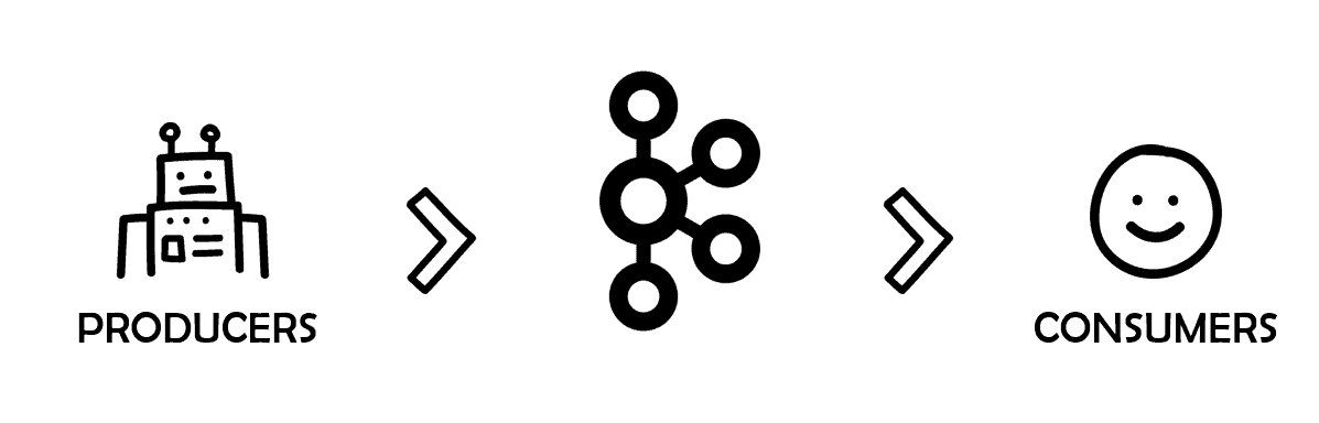
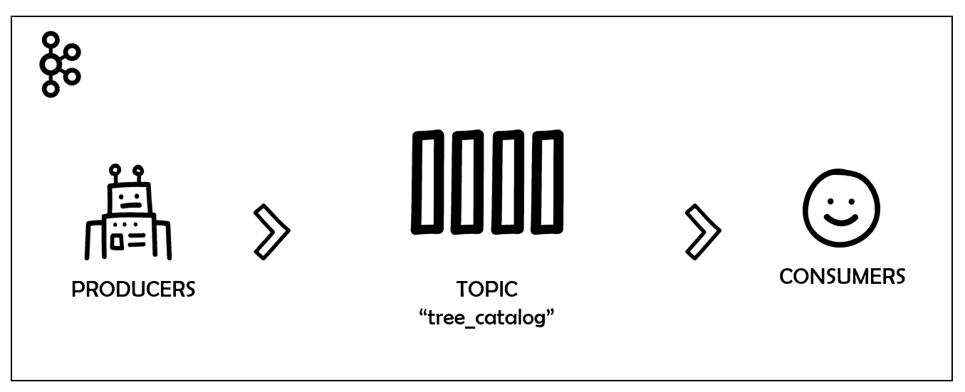
Kafka works as a middleman exchanging information from producers to consumers. They are the two main actors in each edge of this linear process.

Apache Kafka

Figure 1. Producers and consumers in Kafka

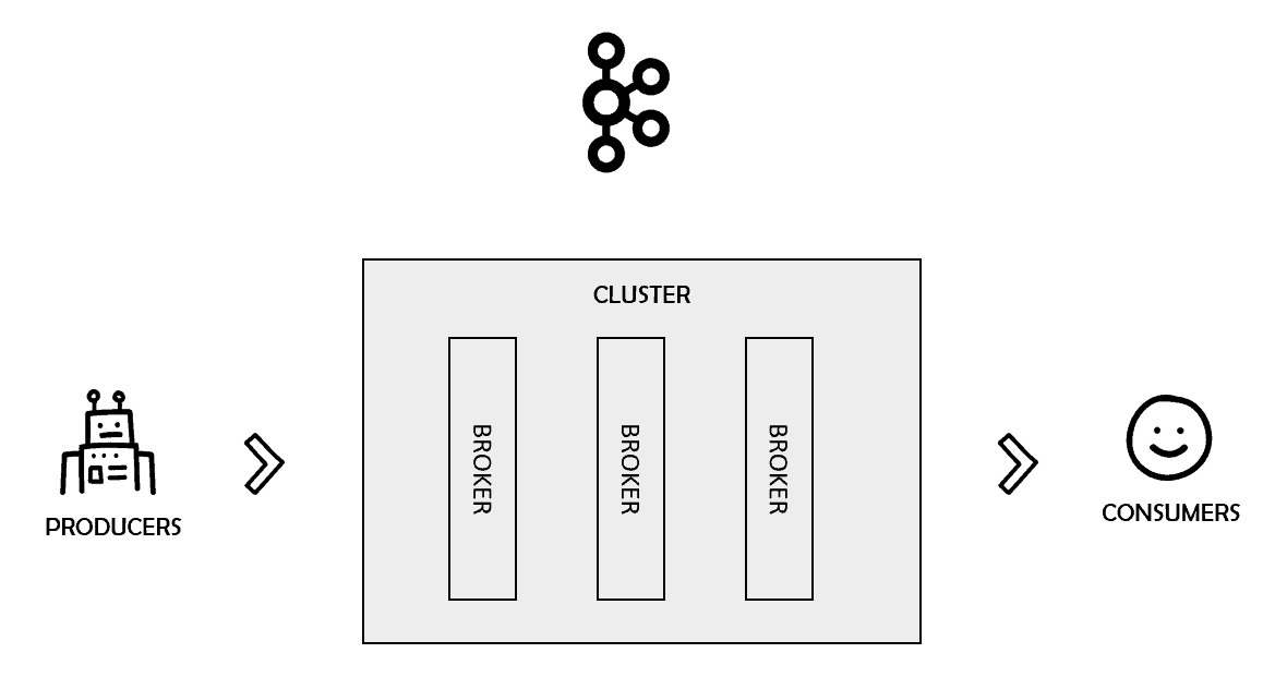
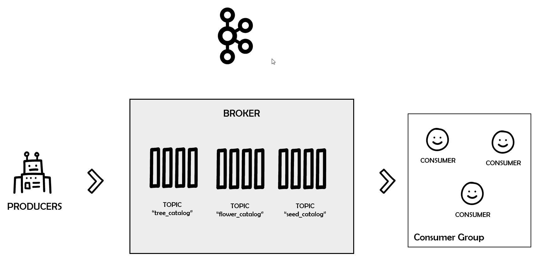
Kafka can also be configured to work in a cluster of one or more servers. Those servers are called Kafka brokers. You can benefit from multiple features such as data replication, fault tolerance, and high availability with brokers.

Kafka clusters

Figure 2. Kafka clusters

These brokers are managed by another tool called Zookeeper. In summary, it is a service that aims to keep configuration-like data synchronized and organized in distributed systems.

Kafka Topics

Kafka is just the broker, the stage in which all the action takes place. The producers send messages to the world while the consumers read specific chunks of data. How do you differentiate one specific portion of data from the others? How do consumers know what data to consume? To understand this, you need a new actor in the play: the topics.

Kafka topics are the channels, the carriage that transport messages around. Kafka records produced by producers are organized and stored into topics.

Imagine that you’re working on a new API project for a catalog of trees and plants. You want to make sure that everybody in the company has access to each newly registered tree. And that is why you picked Kafka.

Every new tree registered within the system is going to be broadcasted via Kafka. The name of the topic is tree_catalog.

Tree catalog in Kafka

Figure 3. Topic tree_catalog in Kafka

In this relationship, the topics work as a stack. It keeps information in the same position as it arrived and guarantees no data loss.

Each data record that arrives is stored in a slot and registered with a unique position number called offset.

When a consumer consumes a message stored in offset 0, for example, it commits the message stating that everything was ok and moves on to the next offset, and so on. The process usually happens linearly. However, since many consumers can “plug” into the same topic simultaneously, the responsibility of knowing which data positions were already consumed is left to the consumers. That means that consumers can decide which order they will consume the messages, or even if they want to restart the processing from scratch (offset 0).

Topic offsets

Figure 4. Topic offsets

Topic Partitions

One key feature of distributed systems is data replication. It allows for a more secure architecture since the data is replicated somewhere else in case bad things happen. Kafka deals with replication via partitions. Kafka topics are configured to be spread among several partitions (configurable). Each partition holds data records via unique offsets.

To achieve redundancy, Kafka creates replicas from the partitions (one or more) and spreads the data through the cluster.

This process follows the leader-followers model in which one leader replica always deals with the requests for a given partition while the followers replicate it. Every time a producer pushes a message to a topic, it goes directly to that topic leader.

Consumer Groups

The most appropriate way to consume messages from a topic in Kafka is via consumer groups.

As the name suggests, these groups are formed by one or more consumers that aim to get all the messages from a specific topic.

To do this, the group must always have a unique id (set by the property group.id). Whenever a consumer wants to join that group, it will do so via group id.

Kafka consumer groups

Figure 5. Consumer groups in Kafka

Every time you add or remove consumers to a group, Kafka will rebalance the load among them so that no overhead happens.

Setup

Now that you know the basics of how Kafka universally works, it’s time to move on to the environment setup. To simplify, the example will use Docker to hold the Kafka and Zookeeper images rather than installing them on your machine. This way, you save some space and complexities.

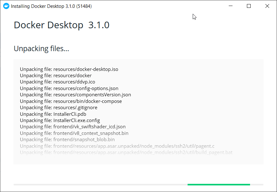
For Windows users, Docker provides a simple way to install and manage your Docker containers: the Docker Desktop. Go to its download page and download the installer. Run it and proceed to the end without changing the default setup options (Figure 6).

Figure 6. Installing Docker on Windows

Make sure to restart your computer after the process is done. After the restart, Docker may ask you to install other dependencies so make sure to accept every one of them.

One of the fastest paths to have a valid Kafka local environment on Docker is via Docker Compose. This way, you can set up a bunch of application services via a YAML file and quickly get them running.

From a code editor (Notepad++, Visual Studio Code, etc.), create a new file called docker-compose.yml and save the contents of Listing 1 into it.

Listing 1. Creating a docker-compose.yml file

version: '2'
services:
  zookeeper:
    image: wurstmeister/zookeeper
    ports:
      - "2181:2181"
  kafka:
    image: wurstmeister/kafka
    ports:
      - "9092:9092"
    environment:
      KAFKA_ADVERTISED_HOST_NAME: 127.0.0.1
      KAFKA_CREATE_TOPICS: "simpletalk_topic:1:1"
      KAFKA_ZOOKEEPER_CONNECT: zookeeper:2181
    volumes:
      - /var/run/docker.sock:/var/run/docker.sock

Notice the code imports two service images (kafka and zookeeper) from the Docker Hub’s account called wurstmeister. This is one of the most stable images when working with Kafka on Docker. The ports are also set with their recommended values, so be careful not to change them.

One of the most important settings of this listing belongs to the KAFKA_CREATE_TOPICS config. Here’s the place where you must define your topic name to be automatically created.

There are other ways to create topics, which you’ll see in the future.

Navigate via the command line to the folder where you saved the docker-compose.yml file. Then, run the following command to start the images:

docker-compose up

This code will start the download of all the dependencies and start the images. During the process, you may see a lot of logs. If no ERROR logs are displayed, then the startup was successful.

Note: You must leave the docker-compose cmd window open, otherwise the images will go down.

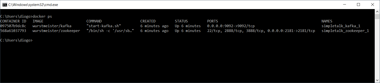
To check if the Docker images are up, run the following command in another cmd window:

docker ps

Figure 7 shows how the output should look.

Figure 7. Checking out the installed Docker images

Hands-on

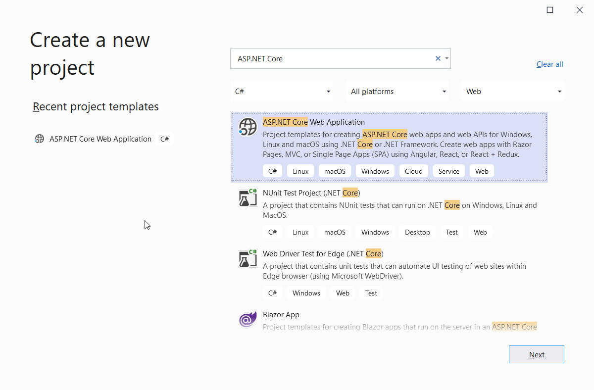
Great! Your Kafka environment is ready to be used. The next step is to jump into the project creation at Visual Studio (VS). Open VS, and head to the project creation window. Search for the ASP.NET Core Web Application template as shown in Figure 8. Click Next.

Create a new ASP.NET project

Figure 8. Creating a new ASP.NET Core Web Application

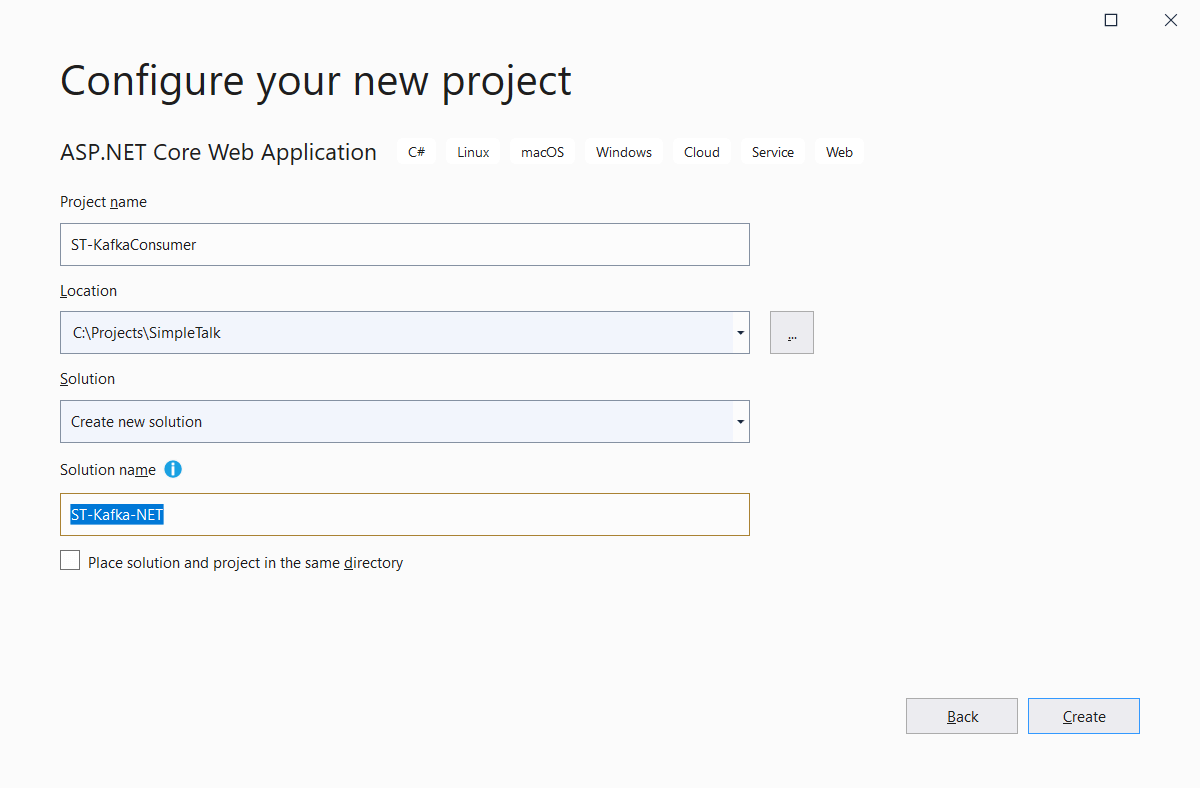
In the following window, make sure to give the solution a different name, as shown in Figure 9. This is because both consumer and producer projects will coexist within the same solution.

Click Create.

Configure your project

Figure 9. Configuring the project and solution names

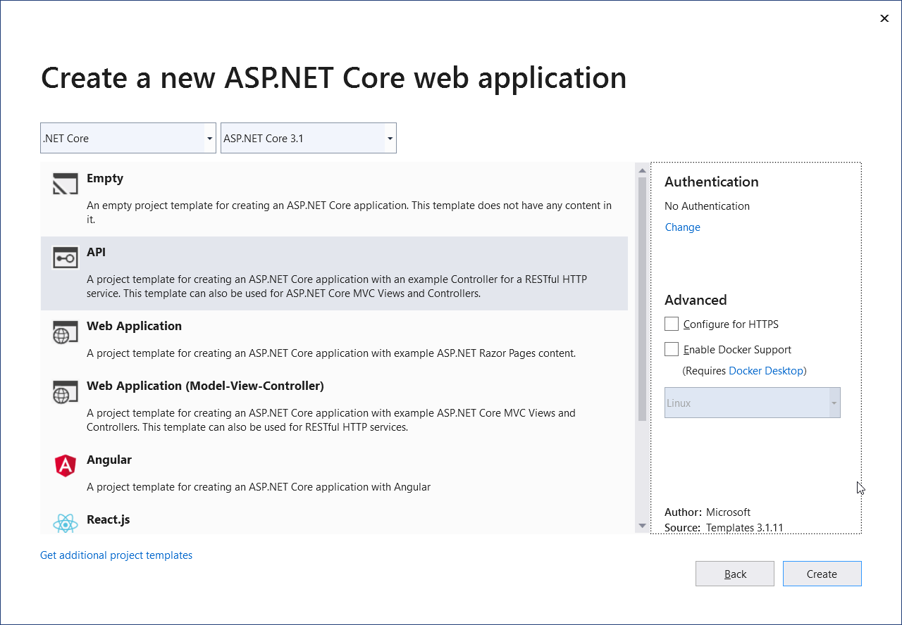
The next window asks for a template selection. Select the API template. Unselect the Configure for HTTPS option. Click Create.

Selecting the project template

Figure 10. Selecting the project template

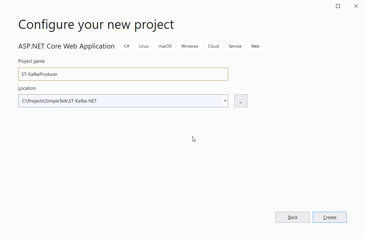
When the project is created, right-click the solution and select the Add > New Project… option. Then, select the same ASP.NET Core Web Application project type and click Next.

Give the project a name like shown in Figure 11.

Creating the producer project

Figure 11. Creating the producer project

Click Create. Go on and select the API template like before, but leave Configure for HTTPS selected. Now, you have two projects in the ST-Kafka-NET solution.

NuGet Packages

To make your C# code understand how to produce and consume messages, you need a client for Kafka. The most used client today is Confluent’s Kafka .NET Client.

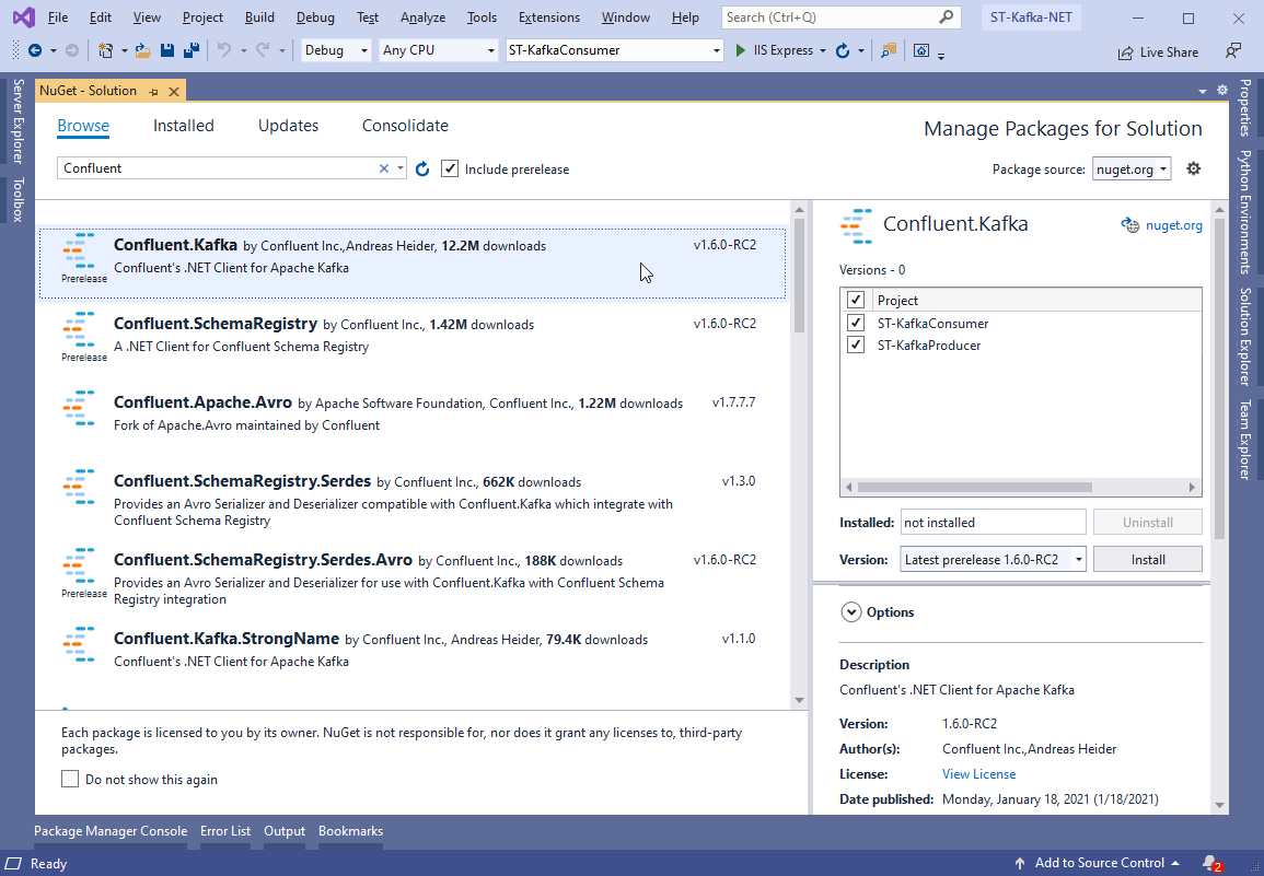
To install it, right-click the solution and select the Manage NuGet Packages for Solution… option. Type Confluent in the search box and select the Confluent.Kafka option, as shown in Figure 12.

Adding Kafka packages to the solution

Figure 12. Adding Kafka packages to the solution

Select both projects and click Install. Alternatively, you can add them via command line:

PM> Install-Package Confluent.Kafka

Setting Up the Consumer

Now to implement the consumer project. Although it is a REST-like application, the consumer is not required. You can have any type of .NET project listening to topic messages.

The project already contains a Controllers folder. You need to create a new one called Handlers and add a new class called KafkaConsumerHandler.cs to it.

Listing 2 shows the new class code content.

Listing 2. KafkaConsumerHandler code

using Confluent.Kafka;
using Microsoft.Extensions.Hosting;
using System;
using System.Threading;
using System.Threading.Tasks;
namespace ST_KafkaConsumer.Handlers
{
    public class KafkaConsumerHandler : IHostedService
    {
        private readonly string topic = "simpletalk_topic";
        public Task StartAsync(CancellationToken cancellationToken)
        {
            var conf = new ConsumerConfig
            {
                GroupId = "st_consumer_group",
                BootstrapServers = "localhost:9092",
                AutoOffsetReset = AutoOffsetReset.Earliest
            };
            using (var builder = new ConsumerBuilder<Ignore, 
                string>(conf).Build())
            {
                builder.Subscribe(topic);
                var cancelToken = new CancellationTokenSource();
                try
                {
                    while (true)
                    {
                        var consumer = builder.Consume(cancelToken.Token);
                        Console.WriteLine($"Message: {consumer.Message.Value} received from {consumer.TopicPartitionOffset}");
                    }
                }
                catch (Exception)
                {
                    builder.Close();
                }
            }
            return Task.CompletedTask;
        }
        public Task StopAsync(CancellationToken cancellationToken)
        {
            return Task.CompletedTask;
        }
    }
}

This handler must run in a separate thread since it will eternally watch for incoming messages within a while loop. Therefore, it’s making use of Async Tasks in this class.

Pay attention to the topic name and consumer configs. They match exactly what was set in your docker-compose.yml file. Make sure to double-check your typing here, since divergences can lead to some blind errors.

The consumer group id can be anything you want. Usually, they receive intuitive names to help with maintenance and troubleshooting.

Whenever a new message is published to the simpletalk_topic topic, this consumer will consume it and log it to the console. Of course, in real-world apps, you’d make better use of this data.

You also need to add this hosted service class to the Startup class. So, open it and add the following code line to the ConfigureServices method:

services.AddSingleton<IHostedService, KafkaConsumerHandler>();

Make sure to import the proper using at the beginning of the class as well:

using ST_KafkaConsumer.Handlers;

Setting Up the Producer

Moving on to the producer, things will be handled a bit differently here. Since there’s no need for infinite loops to listen to messages arriving, the producers can simply publish messages from anywhere, even from the controllers. In a real application, it’d be better to have this type of code separate from the MVC layers, but this example sticks to the controllers to keep it simple.

Create a new class called KafkaProducerController.cs in the Controllers folder and add the content of Listing 3 to it.

Listing 3. KafkaProducerController code

using System;
using Confluent.Kafka;
using Microsoft.AspNetCore.Mvc;
namespace Kafka.Producer.API.Controllers
{
    [Route("api/kafka")]
    [ApiController]
    public class KafkaProducerController : ControllerBase
    {
        private readonly ProducerConfig config = new ProducerConfig 
                             { BootstrapServers = "localhost:9092" };
        private readonly string topic = "simpletalk_topic";
        [HttpPost]
        public IActionResult Post([FromQuery] string message)
        {
            return Created(string.Empty, SendToKafka(topic, message));
        }
        private Object SendToKafka(string topic, string message)
        {
            using (var producer = 
                 new ProducerBuilder<Null, string>(config).Build())
            {
                try
                {
                    return producer.ProduceAsync(topic, new Message<Null, string> { Value = message })
                        .GetAwaiter()
                        .GetResult();
                }
                catch (Exception e)
                {
                    Console.WriteLine($"Oops, something went wrong: {e}");
                }
            }
            return null;
        }
    }
}

The producer code is much simpler than the consumer code. Confluent’s ProducerBuilder class takes care of creating a fully functional Kafka producer based on the provided config options, Kafka server, and topic name.

It’s important to remember that the whole process is asynchronous. However, you can use Confluent’s API to retrieve the awaiter object and then the result that will be returned from the API method. The Message object, in turn, encapsulates the message key and content, respectively. Keys are optional in topics, while the content can be of any type (provided in the second generic argument).

Testing

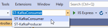
To test this example, you need to run the producer and consumer applications separately. In the upper toolbar, locate the Startup Projects combo box and select the ST-KafkaConsumer option as shown in Figure 13.

Figure 13. Selecting the consumer project to run

Then, click the button IIS Express to run the consumer app. This will trigger a new browser window that we’ll ignore and minimize since the consumer API is not the focus.

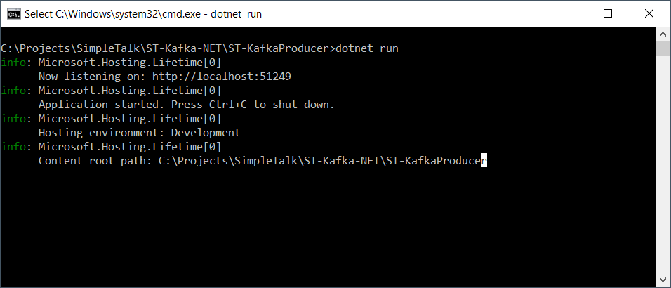
Then, open a new cmd window and navigate to the producer folder. Once there, you can run the command dotnet run to start it up, as shown in Figure 14.

Figure 14. Starting the producer project from the cmd

Pay attention to the URL and port in which it is running.

Now is time to send some messages via producer API. To do this, you can use any API testing tool such as Postman, for example. However, this example will stick to cURL for the sake of simplicity.

For the following commands to work properly, you must ensure that the Docker images are working. So, before running into them, make sure to execute docker ps again to check that out. Sometimes, restarting the computer stops these processes.

If the command doesn’t log anything, run the docker-compose up once more.

To test the publish-subscribe message, open another cmd window and issue the following command:

curl -H "Content-Length: 0" -X POST "http://localhost:51249/api/kafka?message=Hello,kafka!"

This request will arrive at the producer API and trigger the publish of a new message to Kafka.

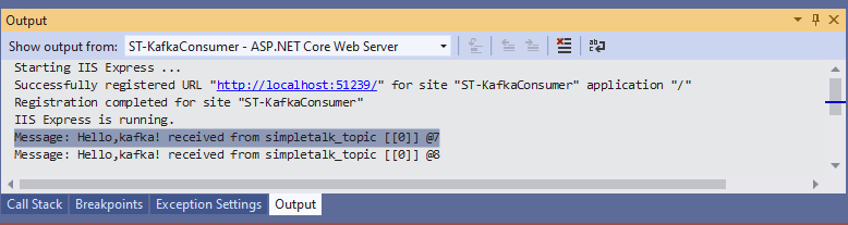
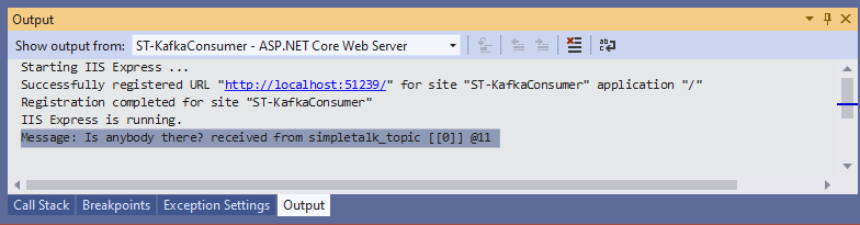
To check if the consumer received it, you may locate the Output window and select the option ST-KafkaConsumer – ASP.NET Core Web Server on the Show output from: combo box, as shown in Figure 15.

Figure 15. Watching consumer logs

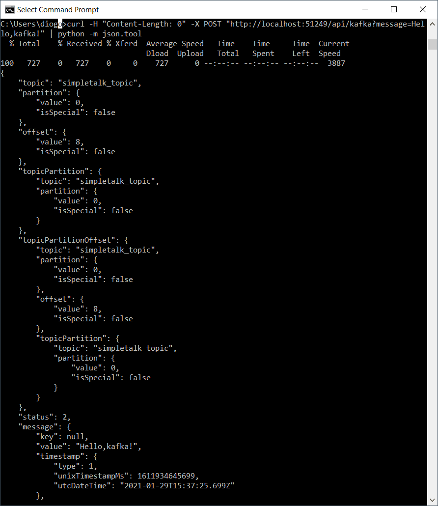
The cmd window may show the JSON result as well. However, it’s not formatted. To fix this, if you have Python installed, you can run the following command:

curl -H "Content-Length: 0" -X POST "http://localhost:51249/api/kafka?message=Hello,kafka!" | python -m json.tool

Which should produce the output shown in Figure 16.

Figure 16. Displaying formatted JSON with Python help

This is all the information about a topic message object you can get for now. A second test will show what happens when the consumer project is down, and a message is published.

Stop the consumer project at Visual Studio and hit another cURL command, but this time with a different message:

curl -H "Content-Length: 0" -X POST "http://localhost:51249/api/kafka?message=Is%20anybody%20there?" | python -m json.tool

Then, start the consumer project again and watch for the logs. You may see the message being consumed right after startup (Figure 17).

Figure 17. The message arriving after startup

Using Apache Kafka with .NET

Pretty nice, isn’t it? What about you? Have you ever used Kafka for your projects? How was your experience with it?

Kafka is a flexible and robust tool that allows for strong implementations in many types of projects, reason number one why it is so widely adopted.

This article was just a brief introduction to its world, but there’s much more to see like Kafka Streams, working in the cloud, and more complex scenarios from the real world. In the next article, I’ll explore Kafka’s capabilities. Let’s go together!


The post Using Apache Kafka with .NET appeared first on Simple Talk.


from Simple Talk https://ift.tt/3auN7cH
via

Wednesday, February 17, 2021

How to become a data scientist: A data-driven approach to careers in data science

Imagine a world without any data. Now imagine the extent of all the available data. Both are equally unimaginable. Every second of the day, petabytes of data are being produced. However, copious amounts of data, also known as big data, in and of itself are not useful until it is computed. As John Allen Paulos famously once said – “Data data everywhere but not a thought to think.”, we are surrounded by an overwhelming amount of data. Still, the real value of having data and analytics teams is in generating this data’s insights. 

Big data needs to be explored, tamed, analyzed, and interpreted before it can be of use. In the recent past, organizations have hired unicorns to help them solve this problem. Unicorns named data scientists that can help them to store, retrieve, and tame their unstructured data. They are also expected to generate predictive insights from the data using advanced analytics.

What does a data scientist do?

Data science combines various disciplines such as data analysis, data engineering, mathematics, statistics, domain expertise, advanced computing, visualization, and much more. A data scientist is expected to have mastery in four fundamental areas: business/domain, mathematics, computer science, and communication.

Thus, a data scientist is someone who can leverage the seemingly infinite amount of data to achieve business goals. They are expected to uncover the latest trends in unstructured data through microscopic attention and analysis. The analysis is followed by effective communication and interpretation of the results, enabling the organization to drive change.

Why is it an exciting time to start a career in data science?

Data science became the rite of passage for many data enthusiasts after the Harvard Business Review called it “the sexiest job of the 21st century”. The field of data science has made enormous strides since this article in 2012. When no universities were offering a degree in data science, Harvard scholars predicted the rapid growth and popularity of this field. Immediately after, LinkedIn saw a rise in the number of people identifying as data scientists.

Data science has been the most sought after career in the US for four consecutive years, according to Glassdoor. Bloomberg reported a 75% increase in job listings for data scientists. In 2018, the demand for data scientists in India shot up by an incredible 417%. According to the US Bureau of Labor Statistics, 11.5 million new jobs are expected to be created in the field of data science by 2026.

Considering the supersonic speed at which data is being produced, the demand for data scientists is not expected to take a dip anytime soon. With technological advancements and the high tide of data submerging every form of industry, organization, and enterprise, it is no surprise that experts who can crunch data are required everywhere. With more and more companies realizing the importance of big data, AI, and machine learning, they are rapidly implementing data science capabilities.

Not just tech for companies, data scientists are being sought by every sector. Tech giants like Amazon, Apple, Facebook, Google, and Microsoft employ only one-half of one percent of the data scientists in the U.S. While there is no shortage of data, there is a shortage of data scientists. According to DataRobot, 73% of organizations surveyed do not have any data scientists or AI specialists.

Since data science is all the rage, it creates a demand for individuals with advanced educational qualifications. All the big organizations look for people with at least a Master’s or a PhD. The higher the educational qualification, the greater is the depth of knowledge required to be a data scientist. According to KDnuggets, 88% of data scientists have a Master’s degree, and 46% have a PhD. However, with an increasing demand for this position and not enough highly qualified professionals to fill them, small companies accept citizen data scientists.

Apart from the high demand and the handsome pay, data science is a satisfying career because of the vast array of problems you can solve with it.

Roles that are close to data science

There are multiple career paths that one could take to become a data scientist. The most obvious route is through education. According to the Bureau of Labor Statistics, most data scientists possess a master’s degree or higher in computer science. Thanks to the diversity of skills required in data science organizations, not everyone needs to get an advanced degree to get into the data science space. There are many paths a working professional can take to become a data scientist. Most of the modern and data-driven organizations have realized the value of data. This realization led to the creation of multiple specialized roles that deliver value using data. Below are some of the data related roles that exist in most organizations:

Data Analyst

A data analyst is required to collect, process, and transform data into usable forms. They help companies make better business decisions. Depending on the organization, an analyst’s job could include tracking web analytics, extracting insights from consumer datasets, analyzing A/B testing, making strategic recommendations based on financial data, or merely organizing messy, unstructured data. A qualified data analyst’s essential requirements are to understand Python, C/C++, HTML, visualization tools, and SQL.

Data Engineer

Data engineers are architects of big data and information pipelines. They strive to create a reliable, interconnected network of data for use within an organization. They design, build, and manage systems that analyze and process data for the organization. They also ensure that the systems run smoothly. This job is different from typical data science careers because it focuses more on hardware and data warehousing than analysis. It is an advanced position and requires a background in software engineering. Data engineers must be skilled in SQL, Databases, Big Data, Cloud computing, Java, Python, Ruby, Matlab, Hive, Pig, SAS, etc.

Database Administrator

Database administrators (DBAs) are responsible for effectively storing and organizing an organization’s data. DBAs are often seen as the guardian angels of the company’s data as they – create highly available databases, design security rules and protocols to safeguard data and perform upgrades to keep databases up to date. DBAs are expected to have at least a bachelor’s degree in computer science or information technology. DBAs are skilled in SQL, Database management, Big Data, Algorithms, Optimization, UNIX/ Linux, Data Analysis, AWS, Python, etc.

Business Analyst

Business Analysis is a great career choice for someone with an educational background in business and a strong foundation in numbers. Business analysis is a less technical position, requiring collaboration between business and IT. A business analyst requires a knowledge of business processes, data visualization tools, and data modeling. They are expected to understand and map out business processes, identify key business problems that can be solved with analytics, and collaborate with other technical groups to translate business problems into solutions.

Business Intelligence Developer

This position requires extensive knowledge about business and the ability to translate data into consumable data products. BI developers and analysts gather data, design and develop systems to increase a business’ efficiency, and help management make good decisions. They do this by either mining data from a company’s software or reviewing competitor data and industry trends. These experts are expected to be tech-savvy, and they can either use the existing BI tools or develop their own BI analytic applications.

Machine Learning Engineer

Machine learning engineers deliver machine learning-focused software solutions to meet an organization’s needs. They design and build machine learning systems that can interpret data and make predictions or draw conclusions. In addition to creating data funnels and machine learning software, they also run tests and monitor the system’s performance to ensure accuracy. These engineers require advanced skills in statistics, programming, and data science.

Data Architect

With the increasing importance of big data, this position is becoming more and more critical. Data architects engineer new database systems, design analytics applications, and create blueprints to integrate, centralize, maintain, and protect data. They ensure the performance of data solutions, improve the functionality of existing systems, and provide access to database analysts and administrators. The position requires a solid understanding of languages like Hive, XML, SQL, Pig, Spark, systems development, and database architecture skills.

How to break into data science?

As I alluded to in the previous section, many roles come close to data science. What are the similarities and differences between these roles? What skills should one add to their profile to become a data scientist? This section will show a data-driven approach explaining the career path options for a citizen data scientist.

Data scientists skills profile

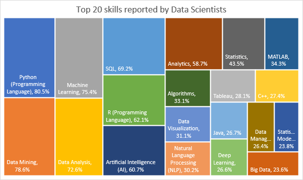
I performed an analysis of the skills that are required to become a data scientist. The information represented below is manually collected from LinkedIn. Figure 1 summarizes the skills of 200 data scientists from leading technology destinations such as the San Francisco Bay Area, New York City Metropolitan Area, Seattle, Dallas-Fort Worth Metroplex, Raleigh-Durham-Chapel Hill Area, Greater Chicago Area, Greater Boston, London Area, Bengaluru, and New Delhi.

Top 20 skills for data science

Figure 1: Top 20 skills of data scientists

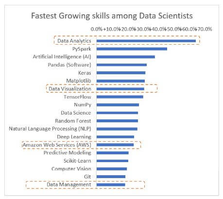
It is abundantly clear from Figure 1 that the top skill that most data scientists have is Python, followed by data mining. Figure 2 represents the fastest-growing skills among data scientists for the last 12 months. It’s interesting to observe that members of other data teams traditionally possess four out of the top 20 growing skills. For instance, “Data Analytics”, and “Data Visualization” skills are very common among Data Analysts, Business Analysts, and Business Intelligence Engineers. “AWS” and “Data management” skills are commonly found among Data Engineers and Database Administrators.

Fastest growing skills for data scientists

Figure 2: Fastest growing skills among data scientists

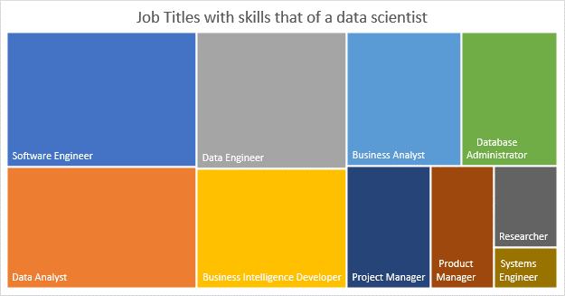
Motivated by these growing skills, I conducted a separate analysis to understand the common job titles of these skills. In other words, I manually collected the job titles of people who have at least one of the top 20 skills that data scientists have. I have excluded data science-related jobs such as Statistician, AI Engineer, ML Developer, etc., from this analysis. Figure 3 summarizes the top 10 job titles for these skills. It is clear from Figure 3 that people who are already in roles such as Software Engineers, Data Analysts, Business Analysts, Data Engineers, Business Intelligence Developers, and Database Administrators have the highest chances of getting into data science.

Job titles with skills that overlap data science

Figure 3: Top 10 Job Titles with skills that of a data scientist

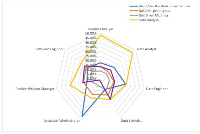
Another data point I looked at is the annual Kaggle Data Science and Machine Learning survey. The latest 2020 survey garnered 20,036 survey responses. The survey attracted global participants at all career and educational levels. This survey asks an extensive list of questions related to their careers, tools usage, nature of work, etc. The specific question that caught my attention is – “Select any activities that make up an important part of your role at work: (Select all that apply)”. The results of this question are summarized in Figure 4. Like the previous analysis, I have excluded data science-related jobs such as Statistician, AI Engineer, ML Developer, etc., from Figure 4. The spider chart from Figure 4 shows that Data Analysts and Business Analysts spend a significant amount of their time performing Data Analysis. Data Engineers balance their time building and running data infrastructure and performing data analysis. DBAs spend a significant amount of their time building and running data infrastructure. DBAs are also seen supporting the data science function by conducting data analysis and assisting the building of ML prototypes. But what’s interesting is the duties of data scientists (yellow line in spider chart). It seems like data scientists are performing duties that are distributed across many skillsets: data analysis, experimentation, ML prototyping, and building ML services. The chart also shows that data scientists spend most of their time performing data analysis than other duties.

Kaggle- Duties performed vs. roles.

Figure 4: Kaggle- Duties performed vs. roles.

Career paths for citizen data scientists:

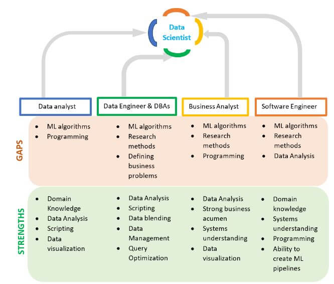
Based on the above data points and analysis, I created four different career paths for citizen data scientists. Data analysts, data engineers & DBAs, business analysts, and software engineers have the most direct career paths to become a data scientist. Figure 5 outlines the options for professionals in data careers to become data scientists and identifies the transferable skills and the gaps that existing data professionals might have to fill.

How to become a data scientist pathways for roles

Figure 5: Career paths for citizen Data Scientists

How to become a data scientist

Data science has become a hot field in the recent past, and it will continue to be one for the foreseeable future. The shortage of people with data science skills will be amplified soon as more companies realize the value of investing in data scientists. This article provides a view into the data science related careers, and it also conducts a detailed analysis of the skills and duties of these related fields. Finally, the article also provides career path options for data professionals to become a data scientist.

If you liked this article, you might also like Building Machine Learning Models to Solve Practical Problems.

The post How to become a data scientist: A data-driven approach to careers in data science appeared first on Simple Talk.


from Simple Talk https://ift.tt/3rYPQB9
via