Saturday, January 15, 2022

Transformations by the Oracle Optimizer

It’s common knowledge that when you write an SQL statement, you’re describing to the database what you want but not how to get it. It shouldn’t come as a surprise, then, that in all but the simplest cases, the statement that Oracle optimizes isn’t necessarily the statement that you wrote. Putting it another way, Oracle will probably transform your statement into a logically equivalent statement before applying the arithmetic it uses to pick an execution path.

If you want to become skilled in troubleshooting badly performing SQL, it’s important to be able to recognize what transformations have been applied, what transformations haven’t been applied when they could have been, and how to force (or block) the transformations you think will have the greatest impact.

In this article, we’re going to examine one of the oldest and most frequently occurring transformations that the Optimizer considers: unnesting subqueries.

The Optimizer’s wish-list

The “query block” is the starting point for understanding the optimizer’s methods and reading execution plans. Whatever you’ve done in your query, no matter how complex and messy it is, the optimizer would like to transform it into an equivalent query of the form:

select  {list of columns}
from    {list of “tables”}
where   list of simple join and filter predicates}

Optionally your query may have group by, having, and order by clauses as well as any of the various “post-processing” features of newer versions of Oracle, but the core task for the optimizer is to find a path that acquires the raw data in the shortest possible time. The bulk of the optimizer’s processing is focused on “what do you want” (select), “where is it” (from), “how do I connect the pieces” (where). This simple structure is the “query block”, and most of the arithmetic the optimizer does is about calculating the cost of executing each individual query block once.

Some queries, of course, cannot be reduced to such a simple structure – which is why I’ve put “tables” in quote marks and used the word “simple” in the description of predicates. In this context, a “table” could be a “non-mergeable view”, which would be isolated and handled as the result set from a separately optimized query block. If the best that Oracle can do to transform your query still leaves some subqueries in the where clause or select list, then those subqueries would also be isolated and handled as separately optimized query blocks.

When you’re trying to solve a problem with badly performing SQL, it’s extremely useful to identify the individual query blocks from your original query in the final execution plan. Your performance problem may have come from how Oracle has decided to “stitch together” the separate query blocks that it has generated while constructing the final plan.

Case study

Here’s an example of a query that starts life with two query blocks. Note the qb_name() hint that I’ve used to give explicit names to the query blocks; if I hadn’t done this, Oracle would have used the generated names sel$1 and sel$2 for the main and subq query blocks respectively.

select  /*+ qb_name(main) */
        *
from    t1
where   owner = 'OUTLN'
and     object_name in (
                select  /*+ qb_name(subq) */
                       object_name
                from   t2
                where  object_type = 'TABLE'
        )
;

I’ve created both t1 and t2 using selects on the view all_objects so that the column names (and possible data patterns) look familiar and meaningful, and I’ll be using Oracle 12.2.0.1 to produce execution plans as that’s still very commonly in use and things haven’t changed significantly in versions up to the latest release of 19c.

There are several possible plans for this query, depending on how my CTAS filtered or scaled up the original content of all_objects, what indexes I’ve added, and whether I’ve added or removed any not null declarations. I’ll start with the execution plan I get when I add the hint /*+ no_query_transformation */ to the text:

explain plan for 
select  /*+ qb_name(main) no_query_transformation */
        *
from    t1
where   owner = 'sys'
and     object_name in (
                select  /*+ qb_name(subq) */
                       object_name
                from   t2
                where  object_type = 'TABLE'
        )
;
select * from table(dbms_xplan.display(format=>'alias -bytes'));

The plan returned looks like this:
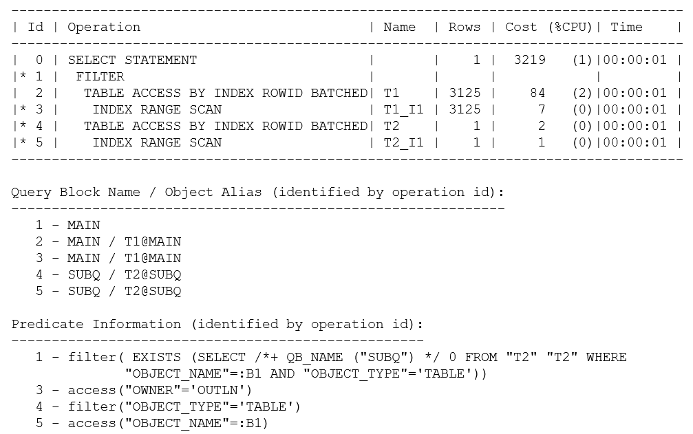
I’ve used explain plan here so that you can see the complete Predicate Information. If I had executed the query and pulled the plan from memory with a call to dbms_xplan.display_cursor(), the predicate information for operation 1 would have read: “1 – filter( IS NOT NULL)”.Since there are no bind variables (and no risk of side-effects due to mismatched character sets), it’s safe to assume that explain plan will produce the correct plan.

There are a few points to pick up on this query and plan:

Even though I have instructed the optimizer to do “no query transformations,” you can see from the Predicate Information for operation 1 that my non-correlated IN subquery has turned into a correlated EXISTS subquery where the correlating object_name has been supplied as a bind variable (:B1). There’s no conflict here between my hint and the optimizer’s transformation – this is an example of a “heuristic” transformation (i.e., the optimizer’s going to do it because there’s a rule to say it can), and the hint relates only to cost-based transformations.

The “alias” information that I requested in my call to dbms_xplan.display() results in the Query Block Name / Object Alias section of the plan being reported. This section allows you to see that the plan is made up of the two query blocks (main and subq) that I had named in the original text. You can also see that t1 and t1_i1 appearing in the body of the plan correspond to the t1 that appeared in the main query block (t1@main), and the t2/t2_i1 corresponds to t2 in the subq query block (t2@subq). This is a trivial observation in this case, but if, for example, you are troubleshooting a long, messy query against Oracle’s General Ledger schema, it’s very helpful to be able to identify where in the query each of the many references to a frequently used GLCC originated.

If you examine the basic shape of this plan, you will see that the main query block has been executed as an index range scan based on the predicate owner = ‘OUTLN’. The subq query block has been executed as an index range scan based on the predicate object_name = {bind variable}. Oracle has then stitched these two query blocks together through a filter operation. For each row returned by the main query block, the filter operation executes the subq query block to see if it can find a matching object_name that is also of type TABLE.

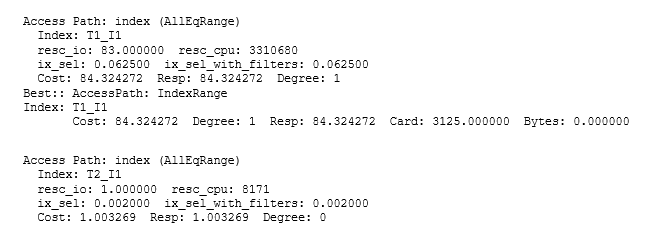
Finally, a comment on Cost: if all you can see is the execution plan, it’s easy to be misled by rounding effects and hidden details of the optimizer allowing for “self-induced caching,” etc. In this case, the base cost of 2 for each execution of the subquery is reduced to 1 in the assumption that the index root block will be cached, and a quick check of the CBO’s trace file (10053 trace) shows that the 1 is actually closer to 1.003 (and the 84 for the t1 access is actually 84.32). Since the optimizer has an estimate of 3,125 rows for the number of rows it will initially fetch from t1 before filtering the total predicted cost of 3219 is approximately: 84.32+ 3125 * 1.003. Realistically, of course, you might expect there to be much more data caching with a hugely reduced I/O load; especially in this case where the total size of the t2 table was only 13 blocks, so a calculation that produced a cost estimate equivalent to more than 3,000 physical read requests for repeated execution of the subquery is clearly inappropriate. Furthermore, the optimizer doesn’t attempt to allow for a feature known as scalar subquery caching so the arithmetic is based on the assumption that the t2 subquery will be executed for each row found in t1.

Here is the section from the CBO’s trace file:
Variations on a theme

The optimizer transformed an IN subquery to an EXISTS subquery. If the value of the object_name in a row from t1 is of interest if it appears in a list of values, then it’s sensible to check by finding that value in the list. If there are duplicates in the list, stop looking after finding the first match. That’s effectively the method of the FILTER operation in the initial plan, but there is an alternative; if the data sets happen to have the right pattern and volume, Oracle could go through virtually the same motions but use a semi_join, which means “for each row in t1 find the first matching row in t2”. The plan would be like the following:
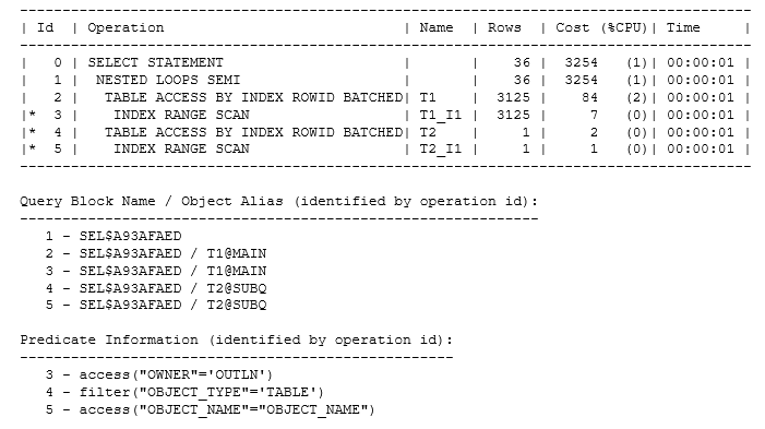
The semi-join was actually the strategy that the optimizer chose for my original data set when I allowed cost-based transformations to take place, but it used a hash join rather than a nested loop join. Since t2 was the smaller row source, Oracle also “swapped sides” to get to a hash join that was both “semi” and “right”:

But there’s more

The volumes of data involved might mean it’s a good idea to adopt a completely different strategy – and this is where unnesting becomes apparent. If the volume of data from t1 is so small that you only have to run the check a few times, then an existence test could be a very good idea (especially if there’s an index that supports a very efficient check). If the volume of data from t1 is large or there’s no efficient path into the t2 table to do the check, then it might be better to create a list of the distinct values (of object_name) in t2 and use that list to drive a join into t1. Here’s one example of how the plan could change:
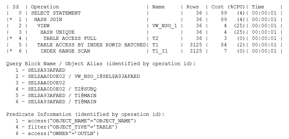
The plan now has a new object at operation 2, a (non-mergeable) view called vw_nso_1 that is recognizably something holding the distinct (hash unique) values of t2.object_name. The number of such values is quite small (only 36 estimated), so the optimizer might have used a nested loop join to collect related rows from t1, but the arithmetic has pushed it into using the “brute force” method of finding all the t1 rows of type TABLE and then doing a hash join.

It’s important to get into the habit of using the alias format option when the shape of the plan doesn’t match the pattern you were expecting to see. In this case, you can see from the Query Block Name information that the final plan consists of two new query blocks: sel$aa0d0e02 and sel$a93afaed. The first query block describes how Oracle will produce a “table” representing the list of distinct object names, and the second query block is a simple join of two “tables” with a hash join. Note how the Object Alias information tells you that the view vw_nso_1 originated in the query block sel$a93afaed.

Side Note: A generated query block name is a hash value generated from the names of the query blocks that were used to produce the new query block, and the hashing function is deterministic.

In effect, the original query has been transformed into the equivalent:

select
        t1.*
from    (
        select
                distinct object_name 
        from    t2 
        where   object_type=’TABLE’
        ) vw_nso_1,
        t1 
where   t1.owner=’OUTLN’ 
and     t1.object_name = vw_nso_1.object_name
/

Whenever you see a view in the plan with a name like vw_nso_{number}, it’s an indication that the optimizer has transformed an IN subquery into an inline view in this way. Interestingly, if you manually rewrite a query to change an IN subquery to an EXISTS subquery, you may find that you get precisely the same plan but with a view named vw_sq_{number}.

And even this strategy could be subject to further transformation if the data pattern warranted it. In my test case, the optimizer does a “distinct aggregation” on a number of small rows before joining to another table to produce much longer rows, which means the aggregation step can be quite efficient. But what if there were a large number of rows to aggregate in t2, and what if the rows were close to being unique and were quite long rows – the aggregation step could require a lot of work for very little benefit. If the join to t1 then eliminated a lot of (aggregated) t2 data and the t1 rows in the select list were quite short, it might be more efficient to join t1 and t2 to eliminate lots of long rows before aggregating to eliminate the duplicates, producing a plan like the following:
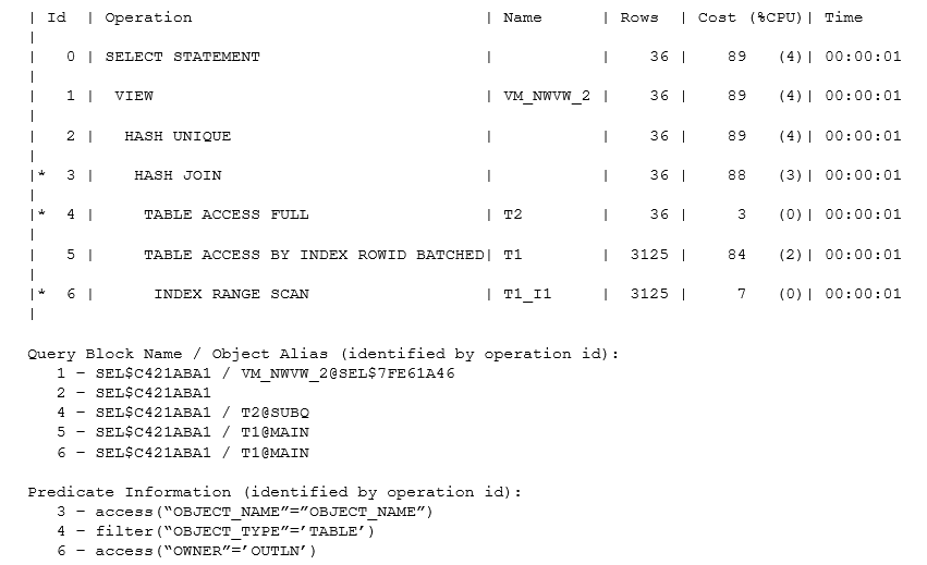
As you can see, the optimizer has produced a hash join between t1 and t2 before eliminating duplicates with a “hash unique” operation. This is a little more subtle than it looks because if you tried to write a statement to do this, you could easily make an error that eliminated some rows that should have been kept – an error best explained by examining the approximate equivalent of the statement that Oracle has actually optimized:

select  
        {list of t1 columns}
from    (
        select 
                distinct
                t2.object_name  t2_object_name,
                t1.rowid _owed,
                t1.*
        from
                t2,
                t1
        where
                t1.owner = ‘OUTLN’
        and     t2.object_name = t1.object_name
        and     t2.object_type = ‘TABLE’
        ) vm_nwvw_2
;

Notice the appearance of t1.rowid in the inline view; that’s the critical bit that protects Oracle from producing the wrong results. Since the join is on object_name (which is not unique in the view all_objects that I created my tables from), there could be two rows in t1 and two in t2 all holding the same object_name, with the effect that a simple join would produce four rows.

The final result set should hold two rows (corresponding to the initial two rows in t1), but if the optimizer didn’t include the t1 rowid in the select list before using the distinct operator, those four rows would aggregate down to a single row. The optimizer sometimes has to do some very sophisticated (or possibly incomprehensible) work to produce a correctly transformed statement – which is why the documentation sometimes lists restrictions to new transformations: the more subtle bits of code that would guarantee correct results for particular cases don’t always appear in the first release of a new transformation.

You’ll notice that the generated view name, in this case, takes the form vm_nwvw_{number} Most of the generated view names start with vw_ this one may be the one special case. The view shows one of the effects of “Complex View Merging” – hence the vm, perhaps – where Oracle changes “aggregate then join” into “join then aggregate”, which happens quite often as a step following subquery unnesting.

Summary

If you write a query containing subqueries, whether in the select list or (more commonly) in the where clause, the optimizer will often consider unnesting as many subqueries as possible. This generally means restructuring your subquery into an inline view that can go into the from clause and be joined to other tables in the from clause.

The names of such inline views are typically of the form vw_nso_{number} or vw_sq_{number}.

After unnesting a subquery, Oracle may apply further transformations that make the inline view “disappear” – turning into a join, or semi-join, or (an example we have not examined) an anti-join. Alternatively, the inline view may also be subject to complex view merging, which may introduce a new view with a name of the form vm_nwvw_{number} but may result in the complete disappearance of any view operation.

I haven’t covered the topic of how Oracle can handle joins to or from an unnested view if it turns out to be non-mergeable, and I haven’t said anything about the difference between IN and NOT IN subqueries. These are topics for another article.

Finally, I opened the article with a discussion of the “query block” and its importance to the optimizer. Whenever you write a query, it is a good idea to give every query block its own query block name using the qb_name() hint. When you need to examine an execution plan, it is then a good idea to add the alias format option to the call to dbms_xplan so that you can find your original query blocks in the final plan, see which parts of the plan are query blocks create by optimizer transformation, and see the boundaries where the optimizer has “stitched together” separate query blocks.

Footnote

If you’ve been examining these execution plans in detail, you will have noticed that all five plans look as if they’ve been produced from exactly the same tables – even though my notes were about how different plans for the same query could appear thanks to different patterns in the data. To demonstrate the different plans, I used a minimum number of hints to override the optimizer’s choices. Ultimately, when the optimizer has made a mistake in its choice of transformation, you do need to know how to recognize and control transformations, and you may have to attach hints to your production code.

I’ve often warned people against hinting because of the difficulty of doing it correctly, but hints aimed at query blocks (the level where the transformation choices come into play) are significantly safer than using “micro-management” hints at the object level.

Although I had to use “micro-management” (object-level) hints to switch between the nested loop join and the hash join in the section “Variations on a Theme,” all the other examples made use of query block hints, namely: merge/no_merge, unnest/no_unnest, or semijoin/no_semijoin.


If you liked this article, you might also like Index Costing Threat

The post Transformations by the Oracle Optimizer appeared first on Simple Talk.


from Simple Talk https://ift.tt/3I3ryOv
via

Tuesday, January 11, 2022

English language confusion

The technology books I’ve written go through a couple of edits, first by someone knowledgeable in the subject area and then by a copy editor. The copy editor will fix misspellings, awkward sentence structure, and grammar. The occasional modification alters the meaning of a sentence, but overall, I’m happy with the updates.

I’ve worked on so many books that the changes by the copy editors are minimal at this point as I’ve learned what types of issues they fix. I was stunned, however, when every instance of “data is” was changed to “data are” in the first edition of my window function book in 2014. I honestly had never heard that the word data was plural or datum, the singular form of the word. There is still quite a debate to be found online, but the consensus seems to be that science articles use data as a plural noun, but use as a singular, collective noun is acceptable.

The English language does evolve over time. We don’t speak like a Shakespearean play or even as people did 100 years ago. Language also ends up different throughout the world or even within a country. For example, in the US, there have been many words to describe a sweet, fizzy drink depending on geography and time: pop, soda, sody pop, tonic, or coke (not necessarily the brand Coke). 

Rules can change, but how do we know when it’s happening? Take the use of “I” vs. “me.” People are in the habit of using “I” after the word “and” regardless of where it ends up in a sentence. You could say “John and I are going to the movies” and be correct since “I” is part of the subject, but “Buy the popcorn for John and I” is wrong because it’s part of the object. The use of “I” after the word “and” in the object of the sentence is so common that I wonder if the rule is changing. It’s easy to use the wrong word when speaking, but I’d expect articles, books, and movies to get it right, which is no longer the case. Now it doesn’t look right to me in the rare situation when I see it used correctly.

Using the correct word is difficult, but spelling in English is even more challenging. Without the electronic tools available today, I would need to carry a heavy dictionary around with me. I’ve never been great at spelling because it requires so much memorization. I’d much rather figure things out than memorize, but there is no figuring out when spelling English words.

The English language frequently doesn’t make sense, so I enjoy writing T-SQL and other programming and scripting languages with dependable features and rules.

Commentary Competition

Enjoyed the topic? Have a relevant anecdote? Disagree with the author? Leave your two cents on this post in the comments below, and our favourite response will win a $50 Amazon gift card. The competition closes two weeks from the date of publication, and the winner will be announced in the next Simple Talk newsletter.


The post English language confusion appeared first on Simple Talk.


from Simple Talk https://ift.tt/3qhnJPA
via

Monday, January 10, 2022

Creating a Database and Tables in PostgreSQL: Learning PostgreSQL with Grant

The series so far:

  1. Connecting to PostgreSQL: Learning PostgreSQL with Grant
  2. Creating a Database and Tables in PostgreSQL: Learning PostgreSQL with Grant

You have an instance of PostgreSQL running locally (or you’re connected to the cloud). Now, what to do with it? In the first article in this series, I said I would start by learning about backups. However, I realized I had another thing I needed to do before I could begin learning – and teaching — backups. I needed to create a database and a couple of tables. I could then back them up.

As with any data management system, there are many ways to get this done. You can do everything from a command line or use a graphical user interface (GUI) that lets you work with PostgreSQL. Finally, the SQL commands are available once you’re connected to PostgreSQL. I’m going to focus there, working primarily within Azure Data Studio (ADS). I’m doing this because:

  1. I like Azure Data Studio. I find it easy to work within. It’s fast. It’s clean. It has plugins to do all sorts of things
  2. For example, it plugs in very nicely to GitHub, so you can easily keep the code as you develop it up on GitHub (go here if you want to see my VERY basic PostgreSQL code: )
  3. I’m old, and I’m just more comfortable working on code within a dedicated coding tool as opposed to simply running it from the command line.
  4. I don’t want to document every single possible method, so I had to pick one. This is it.

That said, let’s get started.

CREATE DATABASE

The command to create a database is quite simple:

CREATE DATABASE postgrelearning;

Well, that was easy.

Let’s talk about this just a little bit. Since I know SQL Server, I’m going to compare what’s going on here, to what’s going on there. In SQL Server, you have a system database called model used as a template when you create a new database. In PostgreSQL, the same thing happens, but the database is called template1. The table template1 operates very similarly to model. You can add objects to template1, and then they will automatically exist in any other new database you create.

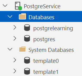
However, there’s more going on in PostgreSQL. Let’s look at my list of databases:

Graphical user interface, text, application, chat or text message Description automatically generated

There’s also a template0 database. What’s that? Well, in the event you completely mess up template1, template0 acts as a baseline. Also, when you restore a database, PostgreSQL uses template0 to start that process (I’ll explain how and why once I learn).

And what about that postgres database? Well, that’s a default built into PostgreSQL so that tools always connect to a default database.

The CREATE DATABASE command has a number of options, as you can see in the documentation. One of the more interesting to me relates right back to those template databases. You can run the CREATE DATABASE command like this:

CREATE DATABASE templatetest WITH template = postgrelearning;

That’s right. You can specify another database as a template. However:

An image showing an error message: source database "postgrelearning" is being accessed by other users

You can only use a database as a template when there are no connections to that database at all.

There are several other options, from defining the database owner, its locale and collation, and more. I’m not going to cover them all now.

If you need to get rid of a database, the command again is simple:

DROP DATABASE templatetest;

That will remove the entire database. However, you can’t have a connection to it when you drop the database. As with CREATE, DROP includes some options. For example, you could write the command like this:

DROP DATABASE IF EXISTS templatetest;

That will eliminate an error if you try to drop a database that isn’t there. Also, you can delete a database that is in use:

DROP DATABASE IF EXISTS templatetest WITH (FORCE);

Now, that’s dangerous, of course. Always exercise extreme caution using this command. In fact, I’d shy away from using it because all it takes is one slip-up, and you’ve dropped the production database.

One more thing. Using ADS, you can quickly and easily switch between databases in the query window. However, there doesn’t seem to be a way to do this strictly from SQL. You control the connection with the tool you are using.

CREATE TABLE

With a database in place, to have something to work with, start by using the CREATE TABLE syntax to get a table in place. If you’re already familiar with an RDBMS, you know that this is a positively huge topic (heck, follow the link and look at the documentation). I’m going to keep it simple for the moment and not go too far down the rabbit hole. There will be plenty to expand on later as we work through this series.

Here’s the first test:

CREATE TABLE TableTest1 
    (ID int NOT NULL, 
    SomeValue varchar(50) NOT NULL, 
    AnotherValue varchar(30) NULL);

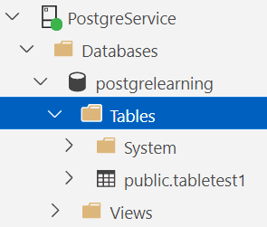
The core syntax is recognizable if you’re coming from SQL Server. The results look like this in ADS:

An image showing PostgreSQL in Azure Data Studio with the Tables folder selected

The code doesn’t include the schema, so the default schema, public, was used. I much prefer to define a schema and then assign tables to that rather than run the default. Having everything in a defined schema or schemas makes it much easier when it comes time to begin to lock things down.

Of course, to really create tables for testing, the example will need to be a bit more sophisticated than the above test. Let’s start with the schema:

CREATE SCHEMA hsr;

From there, create a couple of tables with primary keys and foreign keys:

CREATE TABLE hsr.radiobrand 
    (radiobrandid int PRIMARY KEY GENERATED BY DEFAULT AS IDENTITY,
    radiobranddesc varchar(50) NOT NULL);
CREATE TABLE hsr.radio
    (radioid int PRIMARY KEY GENERATED BY DEFAULT AS IDENTITY,
    radioname varchar(50) NOT NULL,
    radiobrandid int REFERENCES hsr.RadioBrand NOT NULL);

As with SQL Server, there’s syntax to support creating the keys using ALTER as well as CREATE. There’s also syntax for creating a table constraint, which, if you were creating a compound key or consuming one as a foreign key, you’d have to use instead. You could create the hsr.radio table this way:

CREATE TABLE hsr.radio
    (radioid int NOT NULL GENERATED BY DEFAULT AS IDENTITY,
    radioname varchar(50) NOT NULL,
    radiobrandid int NOT NULL,
    CONSTRAINT radiopk PRIMARY KEY (radioid),
    FOREIGN KEY (radiobrandid) REFERENCES hsr.RadioBrand(radiobrandid));

The IDENTITY definition on the column must stay in place since it’s a column property. However, you could create the primary and foreign keys separately from the column definitions. For the sake of consistency, I’ll probably keep that second syntax instead of the first. That way, all the code looks the same, not just some constraints that have compound keys.

That’s the basics.

You can test it out just a little:

insert into hsr.radiobrand
(radiobranddesc)
VALUES
('Icom');
SELECT radiobrandid,
    radiobranddesc
FROM hsr.radiobrand;

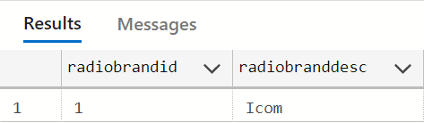
The results are as follows:

An images showing the results of adding a row to the table. Radiobrandid radiobranddesc, 1, Icom

In short, all the basics are working.

Conclusion

We now have a database, a couple of tables, and some data. At its core, PostgreSQL is very much the same as SQL Server. Not identical, of course, but very similar. We’ll start to see more significant differences as we dive deeper. The ability to define more than one template database is a neat trick. The rest of the basics are what I’d expect.

Next time, we really are going to look into backup and restore.


The post Creating a Database and Tables in PostgreSQL: Learning PostgreSQL with Grant appeared first on Simple Talk.


from Simple Talk https://ift.tt/3f9cmTw
via

Data lakes take on big data

The world is generating more data than ever. In 2020 alone, 64.2 zettabytes of data were created or replicated, according to the International Data Corporation (IDC). The IDC also projects that the amount of digital data created over the next five years will be greater than twice the amount of data created since the beginning of digital storage.

Data is being generated on every front—through cloud platforms, mobile computing, edge environments, internet of things (IoT) devices, on-premises data centers, and a variety of other sources—but this data will do little good if organizations don’t have adequate tools for deriving value from it. They need ways to store and access vast amounts of data as efficiently as possible to perform advanced analytics and learn as much as they can from the available information.

To address these challenges, many organizations are turning to data lakes, centralized storage repositories that can hold large amounts of structured, unstructured, and semistructured data in its native format. A data lake offers a flexible and scalable platform for accessing and working with data. It breaks down data silos and addresses some of the challenges of traditional data management approaches. Data lakes are not without their own challenges, however, and organizations should understand their limitations before heading down this path.

What is a data lake?

A data lake is a scalable data storage repository that can quickly ingest large amounts of raw data and make it available on-demand. Users accessing the data lake can explore, transform, and analyze subsets of data as they need it to meet their specific requirements.

One of the most important characteristics of a data lake is its ability to store all types of data from any source:

  • Structured data that is clearly defined and formatted, such as the data found in relational databases.
  • Unstructured data adheres to no specific format, such as social media or data generated by IoT devices.
  • Semistructured data falls somewhere between structured and unstructured data, such as CSV and JSON files.

Early data lakes were built on Hadoop technologies, particularly MapReduce and the Hadoop distributed file system (HDFS). Unfortunately, the first attempts at data lakes often turned into dumping grounds of undocumented and disorganized data, making it challenging to work with the data in any meaningful way. Since then, data lake technologies and methodologies have steadily improved, and they’re now better suited to handle the influx of growing data volumes. At the same time, there’s been a steady growth in cloud-based object storage, which provides a scalable and relatively inexpensive storage platform for handling all that data.

An effective data lake can ingest any type of data in its native format from any source, whether databases, applications, file servers, data streams, or systems such as customer relationship management (CRM) or enterprise resource planning (ERP). A data lake also provides the mechanisms necessary to securely access data and carry out data-related operations without needing to move data to a separate storage system (although this is still an option if required).

Data lakes can help organizations perform advanced analytics that employ techniques such as predictive modeling, machine learning, or deep learning. They can also support business intelligence, making it possible to run queries and generate reports that contain rich visualizations.

A data lake might also be used for warm or cold data that needs to be accessible for compliance requirements or historical analytics. In some cases, an organization might use a data lake as a staging area for a data warehouse, although some organizations use data lakes instead of or alongside data warehouses.

Why use a data lake?

Data lakes offer several advantages. One of the biggest is their ability to support advanced analytics and other forms of data science. Such analytics can help organizations derive greater value from their raw data and open the way for new business opportunities, leading to greater productivity, improved operations, better products, enhanced service delivery, or more effective decision-making.

Data lakes can also help break down silos by providing a centralized repository for storing and working with data from different systems. Data scientists have a complete view of the information, reducing the time needed to identify relevant content, navigate multiple systems, or contend with the various security protections that accompany each system. A centralized repository also reduces the administrative overhead that comes with managing distributed storage.

Data lakes can incorporate any type of data from any source. They’re also highly scalable systems, especially when implemented in the cloud. In addition, data cleansing and transformation are typically performed when the data is needed, rather than when the data is first ingested into the data lake.

These characteristics make the data lake an extremely flexible system that can accommodate a wide range of business needs. Its centralized nature and quick data ingestion enable users to find and respond to information much faster than they can when searching multiple systems. A data lake also makes a wide range of information available to different types of users, providing access to data that was often unavailable in the past.

Challenges using data lakes

Although data lakes can offer numerous benefits, they also come with their own challenges. One of the biggest is the risk that a data lake will turn into a data swamp, serving as little more than a dumping ground for all the data that nobody knows what to do with. The worse the swamp becomes, the more difficult it is for users to find what they need and administrators to track what data is stored in the data lake.

Another challenge is that data lake technologies and processes are still relatively young and have yet to gain the level of maturity available to systems such as data warehouses. Because the data can come in so many formats and types, working with the data can require a wide range of different tools, adding to overhead, complexity, and costs.

This lack of maturity can also lead to data governance challenges, especially with the diversity of tooling and data. In fact, data governance remains one of the top concerns with implementing a data lake. A data lake’s very nature makes governance difficult to achieve, yet that nature also points to the importance of a comprehensive data governance strategy. Without it, the data lake is destined to be plagued by issues in data quality and reliability, making it difficult to carry out the type of analytics needed to make effective business decisions.

Organizations also have to be wary of the unexpected costs that can come with data lakes. Even if an organization uses free, open-source platforms to host the system, there can still be unplanned expenses when it comes to infrastructure and ongoing maintenance, especially if the data lake starts turning into a data swamp. In addition, organizations that rely on cloud storage for their data lakes might experience a degree of sticker shock as subscription fees start to accumulate. Expenses can also add up if IT personnel and other professionals are spending inordinate amounts of time managing and troubleshooting the data lake environment.

Data lake use cases

Data lakes can store large volumes of data, regardless of the type of data or its source. For this reason, a data lake can support a variety of use cases, enabling them to derive meaning from the data through the use of advanced analytics and artificial intelligence technologies such as machine learning and deep learning. Here are just a few of the potential data lake use cases:

  • Education. Educational institutions are continuously collecting data about their students. The data might include information about attendance, grades, test scores, activities or other measures that indicate how well students have done in their academic lives. Through the use of data lakes, these institutions might be able to improve the teaching and learning experience, while increasing student retention and satisfaction.
  • Healthcare. The healthcare industry generates enormous amounts of data in the form of doctors’ notes, patient records, lab test results, clinical trials, administrative documents, and other activities. Data lakes can help the industry derive valuable information from these sources, leading to better treatments and more efficient processes.
  • Financial services. Financial services firms rely on current and accurate data to make decisions as quickly and efficiently as possible. Data lakes can help these organizations derive valuable insights from their data so they can more effectively respond to market trends, predict future outcomes, and reduce overall risks.
  • Climatology. Climatologists can use data lakes to more accurately model and predict the impact of human behavior on the ecology in the short-term and long-term. Data Lakes can also help with research into the steps that can be taken to mitigate the impact on the environment and move toward a more sustainable future.
  • Transportation. Data lakes can lead to more intelligent transportation systems, helping to address a wide range of issues, such as planning traffic flow, scheduling road maintenance, controlling traffic signals, managing road incidents, reducing carbon emissions, deploying fare payment systems, improving crosswalk safety, and numerous other transportation concerns.
  • Telecommunications. Since the onset of COVID-19, telecommunication companies have been under greater pressure than ever to deliver fast and reliable services to support both work-related and personal activities. By implementing data lakes, these companies can better adapt to fluctuating demands and shifts in market trends, while reducing customer churn and dissatisfaction.
  • Cybersecurity. As data continues to be generated at unprecedented rates, cybersecurity continues to be a growing concern. Security specialists can use data lakes to better understand the threat landscape, helping to identify and respond to security threats more quickly and effectively and reduce the risks to sensitive data.

These are by no means the only use cases that might benefit from a data lake. And as the technology and tooling mature, the potential for additional use cases is only likely to grow.

How can you deploy a data lake?

The way in which you go about deploying a data lake depends on the technologies and services you plan to use and where the data lake will be hosted. Regardless of the approach, however, you must take into account how you’ll be moving data into the platform, how you’ll securely store and manage the data and its infrastructure, and how users will be accessing the data.

To get started, you’ll need to have the basic storage infrastructure in place and a defined mechanism for continuously integrating incoming data. You’ll also need a way to effectively handle the metadata that comes with the primary data. Most importantly, you must ensure that security and access controls are built into the system at every step of the way. You should also have a clear sense of how you’ll manage data governance throughout the data lifecycle.

The degree of effort that goes into deploying and maintaining a data lake corresponds directly to the approach you take to implementing the data lake. For example, a cloud service such as AWS Lake Formation helps you build, secure, and manage your data lake, incorporating such features as source crawlers, data transformation, cataloging, security mechanisms, and access controls. AWS Lake Formation also provides built-in integration with Amazon S3 storage, Amazon Athena, Amazon Redshift, and Amazon EMR.

If you try to build a similar system on-premises, you’ll have to deploy a storage infrastructure, a data management platform, a system for ingesting and processing the data, security and access controls, and interfaces for integrating with other systems, tools, and data sources. Even if you use cloud services for all or part of this effort, the do-it-yourself approach can be time-consuming and bring with it additional complexities and overhead, along with mounting costs.

Data lake architecture

There is no fixed formula for a data lake’s architecture. Organizations can combine data lake technologies in different ways to create designs that meet their specific needs while accommodating the influx of heterogeneous data from multiple sources. Even so, data lakes typically share a similar architecture at the highest level, incorporating the following physical layers:

  • Data sources. Data can come from a wide range of sources, including databases, file shares, system logs, business applications, IoT sensors, cloud platforms, NoSQL systems, and many more.
  • Data ingestion. A data lake provides the connectors and other components necessary to rapidly ingest data from the various sources into the storage repository. Depending on the data lake, the ingestion process might also transform or filter the data in some way, but this should not prevent the data lake from ingesting data in its native format from any source.
  • Storage repository. The storage repository is at the heart of the data lake, providing the infrastructure necessary to store various types of data. The repository also stores any associated metadata, which is essential for users to access the data they need easily. Cloud object storage has become one of the most common storage platforms for data lakes, but this is not necessarily a given. The repository can also be implemented on-premises, usually distributed across multiple hosts.
  • Search engine. A data lake requires a scalable, high-performing search engine that enables users to locate and retrieve specific data quickly and easily, no matter how large the underlying data set. For example, a data lake might use Elasticsearch or Cloudera Search to enable users to find data in the repository.
  • Client interfaces. A data lake typically includes APIs or user interfaces for enabling client tools to connect to the search engine, conduct searches and retrieve the results.
  • Client tools. Users can work with a wide range of client tools—running on different devices—to access the data lake environment and its data. For example, they might use data visualization or machine learning tools to work with the data.

Although data lakes commonly store data in its native format, they might also apply formatting to the data in some way, such as converting Excel files to the tab-separated values (TSV) or comma-separated values (CSV). Another approach might be to apply JavaScript Object Notation (JSON) formatting to incoming data. For example, JSON might be used when ingesting data streamed in from IoT devices. A storage repository might also include sandboxed regions to support individual analytics efforts.

Organizations have a great deal of flexibility when building their data lakes, choosing from various tools for implementing the data lake environments and working with the data. They can deploy their data lakes on-premises, on cloud platforms, or in hybrid configurations that accommodate both. Initially, most data lakes were deployed on-premises. Still, the steady increase in the amount of data and the growing availability of cloud object storage have resulted in many organizations moving to the cloud.

Cloud storage services can reduce CapEx and administrative overhead while providing almost unlimited scalability. That’s not to say the cloud doesn’t come with its own challenges, such as mounting subscription fees and lack of control over the environment—a particular concern when it comes to security and compliance—but the cloud makes it possible to deploy a comprehensive data lake platform more quickly and efficiently than trying to do it on-premises—while avoiding many of the headaches that often go with in-house projects.

Data lakes vs. data warehouses

Some organizations operate both data lakes and data warehouses, having clear use cases that justify both. They might use the data lakes as staging platforms for their data warehouses or run them as completely separate systems. Regardless of the scenario, it’s essential to understand the differences between the two approaches to maximize their value and ensure their ongoing success.

A data warehouse is a central repository of structured data that has already been cleansed, transformed, and carefully curated to ensure adherence to the relational database model. This is similar to databases that process transactional operations but with a focus on business intelligence, reporting, and data visualization. In contrast to a data lake, a data warehouse has a very rigid and fixed structure that requires careful planning to implement and change. It also offers limited scalability.

The following table provides an overview of the differences between the data warehouse and the data lake.

Feature

Data warehouse

Data Lake

Types of data

Structured

Structured, unstructured, and semistructured

Schema

Schema-on-write

Schema-on-read

Data quality

Data carefully curated

Data quality can vary significantly

Data volumes

Terabyte scale

Petabyte scale

Agility

Fixed configuration with limited flexibility

Maximum flexibility

Maturity

Very mature features, tools, and security mechanisms

Data lake technologies still maturing

Use cases

Reporting, visualization, and business intelligence

Machine learning, deep learning, predictive analytics, and big data analytics

Users

Business and data analysts

Data scientists, data engineers, and business analysts

Costs

Higher cost per-gigabyte

Lower cost per-gigabyte

Much like data lakes, data warehouses offer both advantages and disadvantages, which is why organizations often implement both. In this way, they can realize the benefits of each system while avoiding some of their challenges. However, implementing two separate systems also requires additional expenses, complexity, and administrative overhead. For this reason, some organizations are now opting for data lakehouses.

A data lakehouse combines data warehouses and data lakes features to create a single platform that offers benefits from both systems. For example, a data lakehouse might support transactions, enforce schema, and provide governance features while using cheaper object storage, handling diverse types of data, and supporting tools typically associated with data lakes. A data lakehouse also reduces data redundancy and the administrative overhead that comes with managing two systems, resulting in lower overall costs.

The growing swell of data lakes

As data volumes continue to grow, organizations will face greater challenges in managing and deriving value from their data. Data lakes can play an important role in bringing order to all that data, but they can provide value only if they help organizations solve business problems and meet their stated goals. For this reason, careful consideration must be given to how a data lake is deployed and maintained and, perhaps more importantly, what the organization hopes to achieve by implementing the data lake.

Data lakes represent a growing presence. Whether they’re used alongside data warehouses, provide staging support for data warehouses, or morph into lakehouses that span both worlds, data lakes could significantly impact how we work with the morass of data expected in the coming years. Data lakes are still relatively new and have a long way to go to reach the maturity level enjoyed by data warehouses. Still, they’ve already gained a strong following, and their popularity continues to grow, especially now that the cloud giants have taken an interest. Data lakes are not for every organization, but for some, they promise to help navigate the challenging waters of data management in the years to come.

If you like this article, you might also like Storage 101: Cloud Storage.

The post Data lakes take on big data appeared first on Simple Talk.


from Simple Talk https://ift.tt/3FbUVwi
via

Thursday, January 6, 2022

Crowdsourcing quality: Can the hive mind/herd mentality help you in software testing?

When I left my employer, 856 people took my place. My job was being done by a village, and not just any village; it was a global village. My role as a software tester was outsourced to a crowd: crowdsourced.

From the time kings invited their populace to try their hand at solving the day’s domestic disturbances, to when the Oxford English Dictionary was compiled from references mailed in by readers, to SETI@home harnessing the power of idle personal computers, crowdsourcing has always been present sometimes hovering in the background, other times appearing in plain sight. Simply put, crowdsourcing means recruiting masses of people of various skills and experiences to perform a certain set of tasks in parallel in a short time.

However, while crowdsourcing seems to work well in situations where user-generated content is useful to build up knowledge, provide first-hand feedback, or raise funds for a good cause, would it also work when it came to improving quality of software? I set out to find more.

The benefits of crowdsourcing software testing

Crowdsourcing testing involves the company hiring amateur and professional testers, assigning them projects to work on, and then paying them (and charging their own customer) according to different pricing models. By far the most popular is pay-per-bug: when a tester reports a bug that the customer agrees to fix, the customer pays the company an agreed amount of money, a small part of which filters down to the tester who found the bug. This amount often depends on the severity and criticality of the bug. With advancements in web communication technology, crowdsourcing testing appears to become an increasingly attractive option in some cases.

Some of the benefits of crowdsourcing testing are:

  • Results drive costs: no results, no money.
  • The crowdsourcing company benefits from on-demand scalability and availability of resources within a short period of time.
  • The customer benefits from a wide variety of skills and talent that may not be available to exploited in-house.
  • Shared product ownership results in brand loyalty and community-building for the greater good.
  • Crowdsourcing is particularly suited to mobile app testing, where there are thousands of OS-Phone-Browser combinations possible making it unfeasible for a single organisation to own so many different products for testing, and simulation is unreliable and risky.

Questions to ask before crowdsourcing software testing

However, there are a number of questions that need to be carefully considered in order to accept crowdsourcing as the next silver bullet of software testing.

Confidentiality: Company projects are confidential. Anyone can join up to test a project and get access to the project information and not much is known or verified about their backgrounds, qualifications, or references. There are no formal vetting checks carried out to ensure that genuine testers are signing on to be part of the project. Sure, you could put hefty NDAs in place, but that knowledge is of little comfort once something of importance leaks and the damage is done. How is confidentiality secured? Does the customer select the testers themselves, or do they have to make do with whoever responds and shows interest in the project? Once assigned, are long-term relationships off-platform (cutting out the middleman) with testers possible?

Business requirements: Crowdsourcing works when the functionality is standard and well known, like an eCommerce sales flow. However, where projects are highly customised and require a thorough knowledge of the customer’s account history, what changes were done and why, and understanding what the customer’s requirements are, how will crowdsourcing random and unknown testers work?

Budget: In smaller companies averaging, say, around 100 bugs per project, at the standard rates for a pay-per-bug model, per project, crowdsourcing may turn out to be very expensive indeed. Could there be scope for cheating, in that the customer could review all the bugs and then decide that they wanted to fix them all but formally accept only a few to keep the costs down? In fact, to keep the costs down, ideally, the customer would want their programmers to only pass on the code to crowdtest after they’re assured of a reasonable level of quality. Does this not imply that there needs to be a certain amount of internal testing done beforehand anyway – either by programmers themselves testing each other’s code, or by an in-house testing team?

Time: There are several time-related issues to consider:

  • Overhead involved for the person(s) who will go through the bug reports, often containing duplicate bugs that need to be filtered out.
  • Overhead in advertising for and then selecting the testers desired for each project.
  • Overhead in creating and providing adequate project documentation for each project – this is especially true and risky for companies that are more agile in their development practices and don’t maintain vast amounts of comprehensive documentation.
  • Delays in communication between programmers and testers if each needs to go through an intermediary. (This also implies loss of traceability if the bugs are logged anonymously, and the programmers don’t know whom to ask for details.)
  • Delays in testing feedback turn-around if bug reports need to be reviewed in-house first by the crowdsourcing company before being released to the customer.
  • Delays in dispute resolution, depending on how much staff is available at the crowdsourcing company to support this.

Bug Quality: Bug reports by testers with varying levels of professionalism may not be accurately worded and meaningful. They may not contain enough information about the bug and its environment, something that comes to experienced professional testers almost as second nature. Worse, some reports may be misleading and time wasters.

Requirements coverage and reporting: What is the guarantee that most testers working on the project won’t focus on the bugs that pay more and thus end up ignoring or leaving unfinished other testing aspects of the project? How does the customer make sure that the entire project scope has been covered fully without having an in-house test manager? Is there provision for traceability to requirements and to draw some progress metrics out from the system?

Agility: For an agile setup where requirements evolve regularly, documentation is kept to a minimum, and communication between team members is key. Crowdsourcing the testing function inherently means a major change in the way the development team works. To ensure that testers understand the full scope and impact of the project, documentation will need to be produced in fine detail with expectations clearly highlighted and transparent. This will also require the investment of resources to keep such documentation up to date. Requirements will have to be frozen and baselined at some point so that the testers can be briefed with reasonable confidence. The testing function will be bolted on at the end of the entire project development lifecycle instead of continuous collaboration with programmers. And finally, communications may break down, either due to time-zone differences not providing an opportunity for direct interaction with the customer representatives, or due to having to wade through a middle-management layer where things can get delayed or lost in translation.

In other words, not agile.

Cultural differences: In a setup where people of different behaviours and work ethics attempt to work together towards achieving a common goal, there is bound to be some uneven interactions. It may be difficult to understand each other’s languages and thought processes. 

Thinking and mindsets vary wildly. At one end of the spectrum is the tester for whom it is perfectly acceptable to challenge a programmer directly or provocatively. Such a tester’s style of communication may be misconstrued as rude or aggressive. At the other end is the tester who may take for granted that they shouldn’t object to anything a programmer says or does out of politeness and respect. Such a tester’s style may be misconstrued as lazy or not proactive.

And what of test data? Where one might find a name like ‘X Æ A-12’ objectionable, another might find it acceptable.

Production environments: When a patch fix for an eCommerce site goes live, company testers put through test orders on the live system to ensure that checkouts and payments have not broken. These test orders are placed in the live system and need to be refunded. Company testers are usually privy to login credentials of several payment gateways. It is virtually impossible for crowdsourced testing to be able to take responsibility for this.

Bigger picture and fit for purpose: Often real value from testing comes not only from detecting bugs but also from being able to look at the entire project at a holistic level, have an overview of the end-to-end business problem and solution and be able to bridge gaps where cracks exist and things have the potential of falling through. With compartmentalised crowdsourced testing, this bigger picture is lost, thus automatically losing a large part of testing effectiveness.

Senior business users who perform user acceptance testing have deep domain expertise. From knowledge and experience, they know which parts of the system are used to what degree, what to review, and in exactly what way. In crowdsourcing, random testers act as users and may not know how the system is intended for use.

Conclusion

If your organisation is looking to crowdsource quality testing as an answer to its prayers, it is worthwhile to carry out due diligence and consider some of the advantages and pitfalls of the concept before making any firm decisions. Conversely, if you own or run a crowdsourcing setup, it pays to be prepared with answers to the most commonly asked questions your potential customers are likely to bring up.


The post Crowdsourcing quality: Can the hive mind/herd mentality help you in software testing? appeared first on Simple Talk.


from Simple Talk https://ift.tt/3zsejUp
via

Wednesday, January 5, 2022

How to replace an identity column with a sequence number

The series so far:

  1. Introduction to SQL Server sequence objects
  2. Using SQL Server sequence objects
  3. How to return multiple sequence numbers with sp_sequence_get_range
  4. How to replace an identity column with a sequence number

Microsoft introduced the sequence number objects starting with SQL Server 2012. A sequence object generates sequence numbers based on starting and increment values, similar to an identity column, but it has additional features. Over time, you might find that the additional benefits of a sequence number have you wanting to replace an identity column with a sequence number. This article demonstrates two options for replacing an identity column with a sequence number.

Why replace the identity column

An Identity column might not be flexible enough to support all business requirements an application might need around a series of identity values. When this occurs, you might find the sequence number object more flexible. Here are a few of the reasons why you might want to change an identity column to a sequence number:

  • Need to know the sequence number prior to inserting a record.
  • Need to share sequence numbers across tables.
  • Need to cycle through a series of numbers, over and over again.
  • Need to retrieve multiple sequence numbers at the same time without gaps.
  • Need to be able to change the specification for the sequence number over time.
  • Need to store a sequence number in a data type other than numeric.
  • Need to allow a sequence number column to be nullable.

Converting identity column to sequence number

If you decide to change an identity column to a sequence number, there is more than one way to accomplish the conversion. This article demonstrates two different options. One option is to modify your table to add a sequence number column and then delete the identity column. Another option is to create another table that uses a sequence object and then use the ALTER TABLE SWITCH operation. This article explores both of these options and provides examples of how these options can be used to replace an identity column with a sequence number.

Option 1: Modify existing table to use sequence number

Replacing an identity column in an existing table using a column populated with a sequence number requires a few steps. To show you how this example works, first create a couple of sample tables.

The first sample table is named Sample and can be created using the script in Listing 1.

Listing 1: Code to create Sample table.

USE tempdb;
GO
CREATE TABLE Sample (ID int identity(1,1) NOT NULL, 
    SampleName varchar(30) NOT NULL,
    CONSTRAINT PK_Sample_ID PRIMARY KEY CLUSTERED(ID ASC));
INSERT INTO Sample(SampleName) VALUES ('First'),
                          ('Second'),
                          ('Third');
SELECT * FROM Sample;

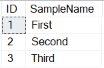
Running the code from Listing 1 produces the rows shown in Report 1.

Report 1: Rows generated in the Sample table

An image showing the results of Listing 1. ID ObjectName 1 First, 2 Ssecond, 3 Third

The Sample table has the identity column that will be changed to use a sequence number.

When swapping out an identity column for a column populated with a sequence number, you need to be careful not to mess up the tables with foreign key references to the identity column of the table being modified. Therefore, this example has a second table named Sample2 created in Listing 2. Sample2 simulates a table with a foreign key reference to the primary key associated with the ID column in the first table.

Listing 2: Creating Sample2 table

USE tempdb;
GO
CREATE TABLE Sample2 (ID int,
CONSTRAINT FK_Sample2_ID FOREIGN KEY (ID) REFERENCES Sample(ID));

Step 1: Creating sequence number column

The first step to replacing an identity column with a sequence number is to create a new column in the Sample table to store the sequence number column. For this example, the sequence number column has the same data type as the original identity column, an INT data type. The code in Listing 3 is used to add the new sequence number column to the Sample table.

Listing 3: Added sequence number column

USE tempdb;
GO
ALTER TABLE Sample ADD SequenceNumber int NULL;
GO

Step 2: Updating SequenceNumber column

Once the new sequence number column has been added to the Sample table, the next step is to update the new column with the appropriate value for all the existing records. The new SequenceNumber column will be populated with the same values as the ID column. Therefore to update the SequenceNumber column, run the code in Listing 4.

Listing 4: Updating the SequenceNumber column

USE tempdb;
GO
UPDATE Sample
   Set SequenceNumber = ID;
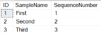
SELECT * FROM Sample;

The output in Report 2 is produced after running Listing 4.

Report 2: Sample table

An images showing the results of Listing 4. ID SampleName SequenceNumber 1 First 1, 2 Second 2, 3 Third 3

Step 3: Identifying and removing foreign key references

The identity column of the Sample table has a primary key named PK_Sample_ID associated with it. This primary key needs to be removed from the ID column and then moved to the new SequenceNumber column. Before this can be done, any foreign keys that reference this primary key need to be dropped. To find all the foreign keys that refer to the PK_Sample_ID primary key, run the code in Listing 5.

Listing 5: Finding all foreign keys

USE tempdb;
GO
SELECT FK.TABLE_NAME as ForeignKeyTable,
      C.CONSTRAINT_NAME as Constraint_Name 
FROM INFORMATION_SCHEMA.REFERENTIAL_CONSTRAINTS C
    INNER JOIN INFORMATION_SCHEMA.TABLE_CONSTRAINTS FK 
    ON C.CONSTRAINT_NAME =Fk.CONSTRAINT_NAME
    INNER JOIN INFORMATION_SCHEMA.TABLE_CONSTRAINTS PK 
    ON C.UNIQUE_CONSTRAINT_NAME=PK.CONSTRAINT_NAME 
    INNER JOIN INFORMATION_SCHEMA.KEY_COLUMN_USAGE CU 
    ON C.CONSTRAINT_NAME = CU.CONSTRAINT_NAME 
    INNER JOIN (
        SELECT i1.TABLE_NAME, i2.COLUMN_NAME
        FROM INFORMATION_SCHEMA.TABLE_CONSTRAINTS i1
            INNER JOIN INFORMATION_SCHEMA.KEY_COLUMN_USAGE i2 
     ON i1.CONSTRAINT_NAME =i2.CONSTRAINT_NAME 
        WHERE i1.CONSTRAINT_TYPE = 'PRIMARY KEY'
    ) PT ON PT.TABLE_NAME = PK.TABLE_NAME
WHERE PK.TABLE_NAME = 'Sample' and PT.COLUMN_NAME = 'ID';

When the code in Listing 5 is run, the output in Report 3 is generated.

Report 3: Output created when Listing 5 is run.

An image showing the result of Listing 5 ForeignKeyTable Constraint_name Sample2 FK_Sample2_ID

To remove the only foreign key identified, the script in Listing 6 can be run.

Listing 6: Removing foreign key

USE tempdb;
GO
ALTER TABLE Sample2 DROP CONSTRAINT FK_Sample2_ID;

Keep in mind any foreign keys dropped should be recreated, so consider retaining the foreign key information.

Step 4: Removing primary key from identity column

With all the foreign keys removed, the primary key on the Sample table can be dropped using the script in Listing 7.

Listing 7: Removing primary key

USE tempdb;
GO
ALTER TABLE Sample
DROP CONSTRAINT PK_Sample_ID;
GO

Step 5: Dropping identity column

With the primary key removed, the identity column can be dropped using the code in Listing 8.

Listing 8: Removing identity column.

USE tempdb;
GO
ALTER TABLE Sample
DROP COLUMN ID ;
GO

Step 6: Renaming SequenceNumber column

For the sequence number column to have the same name as the deleted identity column, it must be renamed. The script in Listing 9 performs this rename operation.

Listing 9: Renaming SequenceNumber column

USE tempdb;
GO
EXEC sp_rename 'Sample.SequenceNumber',
'ID', 'COLUMN';
GO

Step 7: Adding NOT NULL requirement and primary key

Identity columns are defined to have a NOT NULL requirement. Therefore to make the new sequence number column mirror the original identity column properties, the NOT NULL requirement must be added to the sequence number column. The script in Listing 10 alters the ID column to not allow nulls and adds a new primary key constraint to replace the primary key deleted in step 4.

Listing 10: Adding NOT NULL requirement and primary key

USE tempdb;
GO
ALTER TABLE Sample ALTER COLUMN [ID] int NOT NULL;
GO
ALTER TABLE Sample
   ADD CONSTRAINT PK_Sample_ID PRIMARY KEY CLUSTERED (ID ASC) ;
GO

Step 8: Creating sequence number object

Because the Sample table already has some rows, the highest value for the new ID column needs to be determined. This value will be used to set the starting value for the new sequence number object. The starting value for the sequence number object will be the maximum value for the ID column in the Sample table plus the increment value for the sequence object (which in this example will be 1, the same as the original identity increment value). The dynamic TSQL code in Listing 11 can be used to identify the highest ID column value and create the new sequence number object with the correct START value.

Listing 11: Creating Sequence number object

USE tempdb;
GO
DECLARE @NewStartValue int;
DECLARE @IncrementValue int = 1;
DECLARE @CMD nvarchar(1000);
SELECT @NewStartValue = MAX(ID) + @IncrementValue FROM Sample;
SET @CMD = 'CREATE SEQUENCE Sample_SequenceNumber AS INT START WITH ' +
           RTRIM(CAST(@NewStartValue as CHAR)) + 
           ' INCREMENT BY ' + RTRIM(CAST(@IncrementValue AS CHAR));
EXEC sp_executesql @CMD
GO

Care should be used when executing dynamic SQL to ensure you don’t cause a SQL injection issue. Therefore before executing any dynamic SQL, make sure you are not potentially opening the door for SQL injection issues.

Step 9: Setting a default value for the new ID column

When new rows are added to an identity column field, the value for the identity column is automatically populated with the next identity value by default. To get the new ID column to automatically populate with a sequence number value, a default constraint needs to be added to the new ID column. This constraint can be added by using the code in Listing 12.

Listing 12: Setting the ID column default value

USE tempdb;
GO
ALTER TABLE Sample
ADD CONSTRAINT ID_Default 
   DEFAULT (NEXT VALUE FOR Sample_SequenceNumber) FOR ID;
GO

Step 10: Restoring foreign keys

In Step 3, the one foreign key constraint that referenced the primary key on the Sample table was deleted. This step adds back that deleted foreign key reference, using the code in Listing 13.

Listing 13: Restoring foreign key

USE tempdb;
GO
ALTER TABLE Sample2
   ADD CONSTRAINT FK_Sample2_ID FOREIGN KEY (ID) REFERENCES Sample(ID);

Testing out inserting new rows

With the identity column swapped out with a column populated by the sequence number object, all that is left to do is test out the new schema definition. This testing verifies that the new ID column is populated with the next sequence number every time a new row is added. The testing can be done by running the code in Listing 14.

Listing 14: Inserting three new rows into the Sample table

USE tempdb;
GO 
INSERT INTO Sample (SampleName)    
   VALUES ('Fourth'),
          ('Fifth'),
          ('Sixth');
SELECT * FROM Sample;

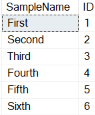
When the code in Listing 14 is run, the results in Report 4 are created.

Report 4: Output when Listing 14 is executed

Image showing the results of running Listing 14. SmpleName ID, First 1, Second 2, Third 3, Fourth 4, Fifth 5, Sixth 6

By reviewing the output in Report 4, you can see that the last three rows inserted got the next three sequential sequence numbers (4, 5, and 6). You might also notice that the position of the ID column is no longer in the first ordinal position in the table as the original ID column was.

Option 2: Replacing identity column using SWITCH operation

Another option to replace an identity column is to use the ALTER TABLE SWITCH operation. This technique is often used with table partitioning, which is out of scope for this article, but it is useful in this scenario. The SWITCH operation doesn’t move the data. Instead, it switches the partition between the source and target tables. This process simplifies the migration, but some requirements need to be followed. Below are those requirements as found in the Microsoft Documentation:

  • Both tables must exist before the SWITCH operation. The table from which the partition is being moved (the source table) and the table that is receiving the partition (the target table) must exist in the database before you perform the switch operation.
  • The receiving partition must exist and it must be empty. Whether you are adding a table as a partition to an already existing partitioned table, or moving a partition from one partitioned table to another, the partition that receives the new partition must exist and it must be an empty partition.
  • The receiving nonpartitioned table must exist and it must be empty. If you are reassigning a partition to form one nonpartitioned table, the table that receives the new partition must exist and it must be an empty nonpartitioned table.
  • Partitions must be on the same column. If you are switching a partition from one partitioned table to another, both tables must be partitioned on the same column.
  • Source and target tables must share the same filegroup. The source and the target table of the ALTER TABLE…SWITCH statement must reside in the same filegroup, and their large-value columns must be stored in the same filegroup. Any corresponding indexes, index partitions, or indexed view partitions must also reside in the same filegroup. However, the filegroup can be different from that of the corresponding tables or other corresponding indexes.

Cleanup and recreating of artifacts from Option 1

Before learning how to use the SWITCH operation to replace an identity column with a column populated with a sequence number, clean the database artifacts created in Option 1 and recreate the sample tables and sequence object. To perform this cleanup and recreation of objects, execute the code in Listing 15.

Listing 15: Cleanup and recreation of sample tables

USE tempdb;
GO
DROP TABLE Sample2;
DROP TABLE Sample;
DROP SEQUENCE Sample_SequenceNumber;
GO
CREATE TABLE Sample (ID int identity(1,1) NOT NULL, 
      SampleName varchar(30) NOT NULL,
      CONSTRAINT PK_Sample_ID PRIMARY KEY CLUSTERED(ID ASC));
INSERT INTO Sample(SampleName) 
   VALUES ('First'),
          ('Second'),
          ('Third');
CREATE TABLE Sample2 (ID int,
CONSTRAINT FK_Sample2_ID FOREIGN KEY (ID) REFERENCES Sample(ID));
GO
USE tempdb;
GO
DECLARE @NewStartValue int;
DECLARE @IncrementValue int = 1;
DECLARE @CMD nvarchar(1000);
SELECT @NewStartValue = MAX(ID) + @IncrementValue FROM Sample;
SET @CMD = 'CREATE SEQUENCE Sample_SequenceNumber AS INT START WITH ' +
           RTRIM(CAST(@NewStartValue as CHAR)) + 
           ' INCREMENT BY ' + RTRIM(CAST(@IncrementValue AS CHAR));
EXEC sp_executesql @CMD
GO

Step 1: Creating new table that uses sequence number

To use the SWITCH operation the target table needs to be created. Use the code in Listing 16 to create the new table that uses a sequence number to populate the ID column instead of an identity specification.

Listing 16: Create a new table

USE tempdb;
GO
CREATE TABLE Sample_New (
   ID int NOT NULL DEFAULT NEXT VALUE FOR Sample_SequenceNumber, 
   SampleName varchar(30) NOT NULL,
   CONSTRAINT PK_Sample_New_ID PRIMARY KEY CLUSTERED(ID ASC)
 );
 GO

Step 2: Removing foreign key references

The SWITCH operation will fail if the primary key on the table being switched is referenced by any foreign keys. Therefore all foreign keys to the Sample table need to be removed first. Sample2 has a foreign key reference to the primary key, which will be removed by running the code in Listing 6.

Step 3: Switching tables

Once all the foreign key constraints have been removed, the SWITCH operation can be performed. The code in Listing 17 will perform the SWITCH operation.

Listing 17: Switch tables

USE tempdb;
GO
ALTER TABLE Sample SWITCH TO Sample_New;
SELECT * FROM Sample_New;

When the switch is performed, the partition between the source (Sample) and target (Sample_New) tables is switched. Only the metadata is changed; the data was not moved. The output of the SELECT statement in Listing 17 can be found in Report 5. This output verifies that rows from the Sample table are now associated with the Sample_New table.

Report 5: Rows in Sample_New table

Image showing results of Listing 17. ID SampleName, 1 First, 2 Second, 3 Third

Step 4: Drop old table and rename new tables

Once the SWITCH operation has been performed, the old Sample table does not contain any rows. Therefore it can be deleted, and the new table can be renamed. The delete and rename can be performed by executing the code in Listing 18.

Listing 18: Drop old and rename new

USE tempdb;
GO
DROP TABLE Sample
EXEC sp_rename N'Sample_New',N'Sample';

Step 5: Recreating deleted foreign key references

The final step of the migration is to recreate the foreign key deleted earlier. This key can be recreated by running the code in Listing 13.

Verifying migration

To verify that this migration was successful, you can run the code in Listing 14. When this code is executed, it should produce the same results as shown in Report 4, with one exception. ID column is now in ordinal position 1. I’ll leave it up to you to run this code and to verify that the SWITCH operation was successful in migrating from an identity column to a column populated with a sequence number object.

Restricting sequence numbers from Being updated

Identity column values cannot be updated, whereas columns populated with sequence numbers can be updated. If you want to make sure sequence numbers cannot be updated, then an AFTER UPDATE trigger will need to be created. To verify that the existing Sample table allows updates to the ID column, run the code in Listing 19.

Listing 19: Updating ID column

USE tempdb;
GO 
BEGIN TRAN
UPDATE Sample
   SET ID = ID + 100;
SELECT * FROM Sample;
ROLLBACK TRAN;
GO

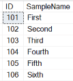
The code in Listing 19 runs successfully and produces the output in Report 6.

Report 6: Output when Listing 17 is run

Image showing results of Listing 19. ID SampleName, 101 First, 102 Second, 103 Third, 104 Fourth, 105 Fifth, 106 Sixth

By reviewing Report 6, you can see that the ID values were all updated from their original values. The code in Listing 19 contains BEGIN TRAN and END TRAN statements to roll back these updates for the next test.

To make sure an UPDATE statement to the ID column in the Sample table cannot be performed, the AFTER UPDATE trigger in Listing 20 needs to be created.

Listing 20: UPDATE trigger

USE tempdb
GO
CREATE TRIGGER trg_UpdateSample
ON Sample
AFTER UPDATE
AS
BEGIN
   SET NOCOUNT ON;
   DECLARE @OriginalID int
   DECLARE @UpdatedID int
   SELECT @OriginalID =[ID] FROM deleted
   SELECT @UpdatedID =[ID] FROM inserted
   IF @OriginalID <> @UpdatedID
   BEGIN
      RAISERROR('Failed: Update performed on ID column', 16, 1);
      ROLLBACK TRANSACTION
   END
END
GO

To test out if this trigger works, run the code in Listing 21.

Listing 21: Testing if trigger keeps ID column from being updated.

USE tempdb;
GO
UPDATE Sample
        SET ID = ID + 100
WHERE ID = 1;
GO

When the code in Listing 21 is run, the error message in Report 7 is produced

Report 7: Error when Listing 21 is executed

Image showing error message after running Listing 21. Msg 5000 Level 16, State1. Procedure trg_UpdateSample Line 13 (Batch start line 2) failed: update performed on ID column. The transaction ended in the trigger. The batch has been aborted.

By creating the AFTER UPDATE trigger trg_UpdateSample, the code in Listing 21 could not update the ID column.

Replacing identity an column with a sequence number

Over time, you may find out that an identity column needs to be swapped out and replaced with a sequence number. This article provided a couple of examples of how to perform that swap. If you plan to replace an identity column with a column populated with a sequence number value, keep in mind sequence number columns can be updated. To restrict sequence columns from being updated, an AFTER UPDATE trigger needs to be defined to restrict the updates.

The post How to replace an identity column with a sequence number appeared first on Simple Talk.


from Simple Talk https://ift.tt/34acG1Z
via

Monday, January 3, 2022

Evaluation policies in a tenant-wide level and more Azure tricks

I wrote many blogs about policies in Azure. I started talking about How essential Policies are, than including them in a blog about Azure SQL AD Only Authentication  and finally about how to ensure Azure SQL is with Azure AD Only Authentication enabled. 

Using both, policies and management groups, we can manage standards across a word-wide company tenant. We can create policies on many hierarchical levels and apply them.

When we create new policies and assign them to a management group, we may would like to have an evaluation of these policies, know the compliance of the existing objects.

We can manually trigger this evaluation even in a world-wide level. The evaluation is always triggered on a resource group level.

Manually Triggering the Policies

That’s what I’m including on this post: A powershell script to trigger the policy evaluation for all resource groups in our company.

The resource groups may be in different subscriptions. We will need to list the subscriptions and execute the evaluation for the resources groups on each subscription at a time.

For this, I will use another trick I already wrote about many times: KQL – Kusto Query Language.

You may would like to check some articles I wrote about KQL:

Microsoft built a layer on Azure background called Azure Resource Graph. Azure Resource Graph allow us to use KQL to query Azure Resources.

We can execute a KQL query in Powershell to retrieve the objects we need to deal with, then we process these objects. This can make some powershell code way easier.

The script below does this task

  1. Retrieves the subscriptions from Azure
  2. Loop through the retrieved subscriptions
  3. For each subscription, change Azure context to it
  4. Get all resource groups
  5. For each resource group, start the processing of the policies as a powershell job

Write-Host "Starting"
$result=(Search-AzGraph -Query 'resourcecontainers
| where type == "microsoft.resources/subscriptions"
| project name, subscriptionId')

$result | foreach {

   Write-Host "changing subscription to $($_.subscriptionId)"

   Set-AzContext -Subscription $_.subscriptionId
   
   Get-AzResourceGroup | foreach {
                Write-Host "starting $($_.ResourceGroupName)"
                Start-AzPolicyComplianceScan -ResourceGroupName $_.ResourceGroupName -AsJob
                }

}


Executing the Script

This script doesn’t care about the azure authentication because it’s built to be executed inside the Cloud Shell. In this way, the authentication will already be present and the script works exactly as it is now.

The cloud shell can make things even easier for us. It’s linked to a File share in a storage account. We can create a map of this file share in our local machine and use it to create and edit scripts like this one on your local machine and directly save them to the cloud shell.

The post Evaluation policies in a tenant-wide level and more Azure tricks appeared first on Simple Talk.


from Simple Talk https://ift.tt/32CHAjn
via