Thursday, May 18, 2023

PostgreSQL Basics: A Template for Managing Database Privileges

In the first two articles of this series about PostgreSQL privileges, we reviewed how to create roles, grant them privileges to database objects, and how object ownership is an important aspect in managing access and control within the database.

When it comes to managing what roles can access or modify an existing object, ownership is the ultimate privilege. Because PostgreSQL privileges work from a Principle of Least Privilege mindset, the owner of an object (table, trigger, function, procedure, etc.) needs to GRANT privilege to other roles.

We discussed how this can be done manually with a GRANT command each time an object is created, however, that is time consuming to manage and easy to miss a detail.

Instead, PostgreSQL provides a method for setting default privileges which are granted on behalf of the object owner as database objects are created. Using default privileges, a role can prepare the database ahead of time to ensure that consistent access privileges are applied while easing the management burden over time.

But how do you go about creating a set of roles and default privileges that will provide the right level of control and access? Let’s dig a little deeper.

Using Default Privileges to Manage Migrations

Recall that default privileges are set per role (which can represent a user or a group of users). That is, each role must specify what privileges it will grant to other roles whenever a specific type of object is created. Consider the image illustration below of a database with a number of objects inside, each owned by a different role.
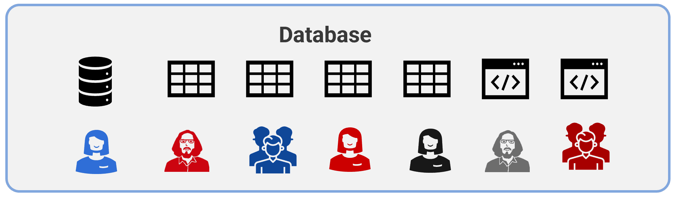
A picture containing diagram Description automatically generated

A database that allows many roles to create and own objects introduces at least two issues.

First, it means that many roles have the CREATE privilege in each schema. As we discussed in the previous articles, object creators are also the owners by default and have a superuser-like privilege for the object. More than that, however, having the privilege to create objects in a schema creates a potential security issue, the very reason the CREATE privilege was removed from the public role in PostgreSQL 15.

Second, even if you have legitimate reasons for many different roles to create objects in a schema, each of them will need to create and maintain a set of default privileges to ensure the other roles have the access they need. That’s a lot to manage, even more so because it’s challenging to easily visualize default privileges in PostgreSQL, currently.

Instead, consider this second illustration, showing one group role that owns all database objects. In this scenario, the group role cannot login which provides some level of security, and only one set of default privileges must be maintained over time to manage access of database objects and data effectively and efficiently.
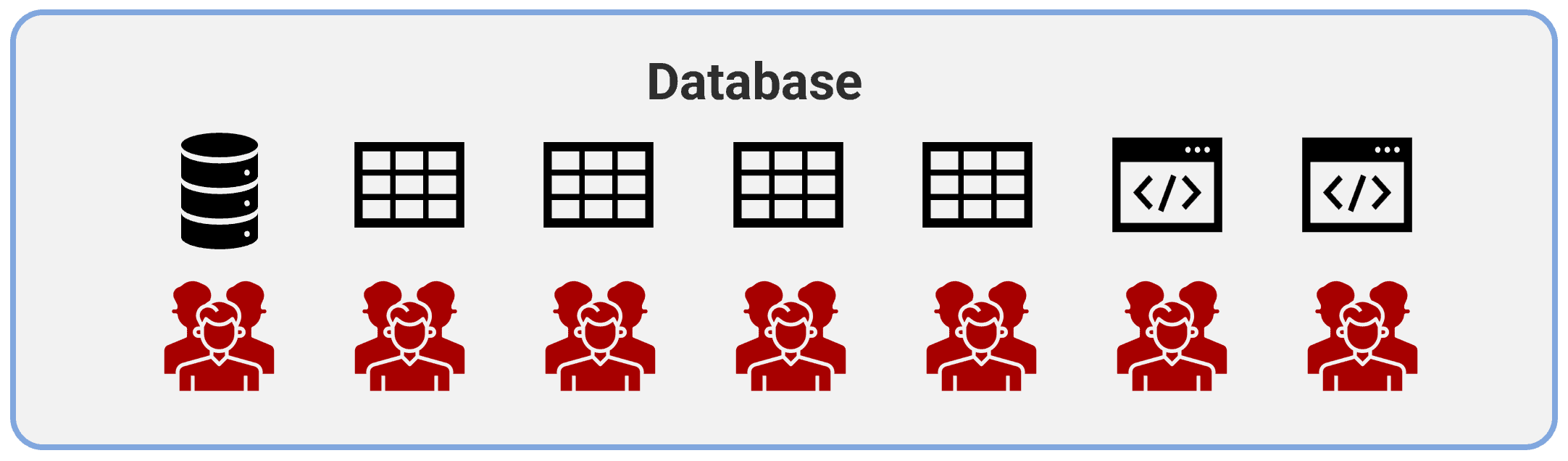
Diagram Description automatically generated

Let’s look at how you can start to move towards this kind of security set up within your PostgreSQL databases.

Create High-level Group Roles

In PostgreSQL, roles can be granted membership in other roles and inherit their privileges, something we discussed in the first article. The challenge, then, is to think about the kinds of privileges you need to provide to different roles in your database and how to abstract them into higher sets of roles.

Remember that roles are created at the instance level. Therefore, if you create a ‘read_only' role, it can be used to manage read-only access ('SELECT') in each database. The same can be done with different kinds of privileges from DML access (‘INSERT', ‘DELETE', ‘UPDATE') all the way up to DDL operations (‘CREATE').

A sample “template”, then, can start by creating these three group roles in every database instance. Your needs may be more complex, so please add and adjust as you see fit.

  • The following scripts are a modified version of this Stack Overflow answer to use as a template. I happened upon it last year and thought it does a good job outlining a straightforward process to setting up PostgreSQL database privileges. (It doesn’t hurt that it mentioned the best Database DevOps tool as well! 😊)

PostgreSQL Instance Group Roles

The following two scripts need to be run once on each database instance to create the appropriate roles which we will then be granted privileges within each database.

/*
* This script should be run ONCE per PostgreSQL instance
* to create the group roles that will/can be used in all databases
* for ddl/dml/read_only access 
* 
* In your situation, you may need to create more group roles to
* provide better granularity of privileges.
*/
CREATE ROLE ddl_grp WITH NOLOGIN;
CREATE ROLE dml_grp WITH NOLOGIN;
CREATE ROLE read_only_grp WITH NOLOGIN;

Creating these roles hasn’t done anything of substance, yet. Instead, these roles become a mechanism to manage other privileges as we create a database and schema objects. Even though you cannot connect to a database directly with these roles ('WITH NOLOGIN'), these roles can still own objects and create default privileges.

Next, we can grant membership into these group roles to other roles as necessary. In the example below, we have three types of user roles:

  • Object admins: these roles are allowed to create objects in a database. Creating objects is a DDL action, so we named the role 'ddl_grp'
  • Data admins: these roles are allowed to modify data and associated objects with DML statements, so we named the role ‘dml_grp'
  • Read-only: these roles are allowed to select data from specific schemas or tables. We named the role ‘read_only_grp'

The examples user roles (eg. 'dev_admin1', ‘flyway', ‘dev1', ‘report_usr', etc.) need to exist prior to granting membership in the group role. The key is that any role that is granted membership to the ‘ddl_grp' role will be able to run scripts that create or modify objects in the database as ‘ddl_grp'.

/*
 * Now, grant access to each role as necessary for their
 * job function. Again, these are just ideas of how to get
 * started. More "group" roles may be necessary
 * 
 * These are example roles that might be given access. A good
 * example of a role that should be in the "ddl_grp" is the
 * role that is used by DevOps tools like Flyway to run
 * migrations scripts. This ensures that all objects are owned
 * by that group and all users get access.
 */
GRANT ddl_grp TO dev_admin1, flyway;

GRANT dml_grp TO dev1, dev2;

GRANT read_only_grp TO report_usr1, report_usr2;

With all roles in place and membership updated, we can now turn to the individual database where privileges really matter.

Individual Database Privileges

Now that we have the database roles created, we can focus on the individual database privileges. In this case you have two options.

You could run this script each time a new database is created in the cluster. Or, using a superuser role, you can modify the template database (typically called ‘template1') on your PostgreSQL instance. Any settings that are applied in the template database will automatically set these privileges for each new database that is created from that template.

The script below can be applied as one script, however, I’ve broken it apart to discuss the purpose of each section and how it applies to the database.

Revoke all privileges from PUBLIC

The first thing that should be done for any new database is to revoke all privileges that are granted by default to the PUBLIC role. We discussed in the first article why this is a recommended practice.

/*
 * On EACH database, run this script as a superuser or
 * user that has CREATEROLE and other GRANT privileges.
 * In a DBaaS service like Amazon RDS, this may be a user
 * that was assigned to you for administration
 */
-- For all modern versions of PostgreSQL. This will
-- prevent connections to the database until specifically
-- granted with CONNECT
REVOKE ALL ON DATABASE mydatabase FROM PUBLIC;

-- Prevent anyone from creating objects in the public
-- schema until granted permission. Default on PG15+
REVOKE CREATE ON SCHEMA public FROM PUBLIC;

Notice one nuance here. We are removing ‘ALL' privileges from 'PUBLIC' at the database level, not the schema level of the database. If we removed all privileges from the schema as well, then normal PostgreSQL commands would not work for many users without resetting additional privileges.

Revoking 'ALL' at the database level prevents users from connecting to the database without specific grants applied elsewhere, as shown below.

Grant basic privileges

All roles need the ability to connect to the database and (typically) access temporary tables. However, without additional privileges like USAGE and SELECT, these roles can’t actually do anything in the database yet.

Normally every role would inherit these privileges from the PUBLIC role, but we just revoked those privileges above to give us more control over which roles we want to access each database and the public schema.

-- GRANT connect and access to all roles;
GRANT CONNECT, TEMPORARY 
        ON DATABASE mysuperdb TO ddl_grp, dml_grp, read_only_grp;

Grant usage and other privileges to each group role

Now we get to the good stuff. For each database we can decide which roles can use the database objects ('USAGE') and what they can do per schema. As noted below, this example only shows how to grant privileges on the public schema. If your application has other schemas (which it probably does!), you will need to grant the appropriate permissions on each schema.

First, our 'ddl_grp' (and all members) is allowed to use and create objects in the schema and any sequences. If there are existing objects such as TABLE, SEQUENCE, TYPE, DOMAIN, etc. you do need to run a GRANT statement for each time to set their existing privileges appropriately because default privileges only effect newly created objects. In the example below, I show granting privileges to existing sequences and tables.

/*
 * Below, we grant usage on an application schema called 'myapp'.
 * If your application has a different schema, you will need to
 * update this appropriately. 
 * 
 * Multiple schema names can be separated by a comma  
 */
-- This will allow anyone in the group to use and create
-- new objects in the schema. Because this group will own
-- the objects, they can modify them later.
GRANT USAGE, CREATE
    ON SCHEMA myapp TO ddl_grp;

-- modify privileges for any existing tables and sequences
GRANT ALL
    ON ALL TABLES IN SCHEMA myapp TO ddl_grp;

GRANT ALL
    ON ALL SEQUENCES IN SCHEMA myapp TO ddl_grp;

Next, we move on to the group roles that will be allowed to use objects in a schema and then select data and sequence values. As before, if your database has multiple schemas, the roles will need to be granted usage for each object type in each schema.

-- This will allow all other "group" roles to connect
-- to the myapp schema and access objects if they have
-- have been granted privileges to do so.
GRANT USAGE ON SCHEMA myapp TO dml_grp, read_only_grp;

-- modify privileges for any existing tables and sequences
GRANT SELECT
    ON ALL TABLES IN SCHEMA myapp TO dml_grp, read_only_grp;

GRANT USAGE, SELECT
    ON ALL SEQUENCES IN SCHEMA myapp TO dml_grp, read_only_grp;

Finally, as the user that will be used to create schema objects, set the default privileges for other roles in the database. Notice two things in the following example.

  • We only set default privileges for tables and sequences. You should consider other privileges that your users will need as objects are created and add them to your script.
  • The 'ddl_grp' role doesn’t have any default privileges assigned, nor to any of the roles which are members of it. This is because the group will be the owner of the object and any other member role will automatically inherit the ownership privileges. Nothing more is needed.

Default privileges are normally applied to the role that executes the statement. Therefore, your scripts must temporarily set the role to the owner that will create objects in the future. This requires that the role executing this script is a member of the other role.

Alternatively, and slightly clearer in the long run, you can set the default privileges for another role as part of the ALTER DEFAULT PRIVILEGES statement as long as the current role is a member of it.

In both examples below, the role that is executing the SQL must be a member of the other group role. The second form is a bit more verbose and easier to track at a statement level what privileges are being applied to whom.

Option 1: SET ROLE before assigning privileges

/*
 * Finally, as the user that will run migration scripts (and is
 * a member of the DDL group, setup the default access privileges.
 */
SET ROLE ddl_grp;
ALTER DEFAULT PRIVILEGES IN SCHEMA myapp
GRANT SELECT, INSERT, UPDATE, DELETE ON TABLES TO dml_grp;

ALTER DEFAULT PRIVILEGES IN SCHEMA myapp
GRANT SELECT ON TABLES TO read_only_grp;

ALTER DEFAULT PRIVILEGES IN SCHEMA myapp
GRANT USAGE, SELECT ON SEQUENCES TO dml_grp, read_only_grp;

ALTER DEFAULT PRIVILEGES IN SCHEMA myapp
GRANT UPDATE ON SEQUENCES TO dml_grp;

Option 2: Assign privileges for another role

/*
 * Finally, as a user that has membership in the group role that
 * will run migration scripts setup the default access privileges.
 */
ALTER DEFAULT PRIVILEGES FOR ROLE ddl_grp IN SCHEMA myapp
GRANT SELECT, INSERT, UPDATE, DELETE ON TABLES TO dml_grp;

ALTER DEFAULT PRIVILEGES FOR ROLE ddl_grp IN SCHEMA myapp
GRANT SELECT ON TABLES TO read_only_grp;

ALTER DEFAULT PRIVILEGES FOR ROLE ddl_grp IN SCHEMA myapp
GRANT USAGE, SELECT ON SEQUENCES TO dml_grp, read_only_grp;

ALTER DEFAULT PRIVILEGES FOR ROLE ddl_grp IN SCHEMA myapp
GRANT UPDATE ON SEQUENCES TO dml_grp;

Verify the privileges are set correctly

The last step is to verify that the default privileges are set and ready to do their job. The easiest way to see the result of your work is with the ‘\ddp’ command in ‘psql’.
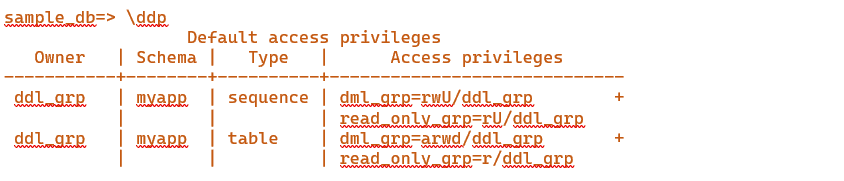
A close-up of a computer code Description automatically generated with low confidence

This helps us verify that the 'ddl_grp' role set default privileges for all tables and sequences in the public schema.

Obviously, your application and role set up is probably more complex than this example template. However, the principles apply regardless of how many roles and object types you need to manage. Use this as a starting point.

Bringing It Together At Migrations Time

With everything in place, let’s look at how you would use this in practice on a production database (for example).

In the migration pipeline, we set the connection string for the migration script to use our pipeline role, shown as “flyway” above. Ideally, the password for this role would be stored in a vault and is retrieved as part of the pipeline script so that no regular user can authenticate as this role.

At the top of any migration script, then, we first set the role to the 'ddl_grp' role so that any creation DDL will cause the objects to be owned by that group and the default privileges will kick in and be applied correctly! A simple example might look something like this.

/*
 * First set the session role to the high-level 
 * ownership group role
 */
SET ROLE ddl_grp;

-- Create the object
CREATE TABLE test (
    col1 text null,
    col2 int null
);

Once the migration has been applied, you can quickly check that the privileges were applied correctly using the '\dp' command in '\psql'.
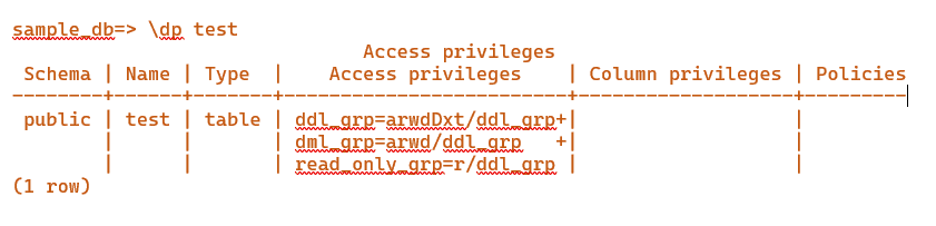
A close-up of a code Description automatically generated with low confidence

Success! From this point forward, as long as the 'ddl_grp' is used to create tables and sequences (or any other objects that you set default privileges for), other roles will have the access you defined, and the overall management burden is reduced!

Conclusion

Privileges in PostgreSQL can be complex to think about and manage. Knowing how to grant privileges to roles and membership between roles can quickly improve this burden. However, learning how to setup default privileges in an effective way is where the real power of managing your database begins.


The post PostgreSQL Basics: A Template for Managing Database Privileges appeared first on Simple Talk.


from Simple Talk https://ift.tt/dGFe4nr
via

Monday, May 15, 2023

Changing log growth strategy in SQL Server 2022

When I first saw a bullet item stating SQL Server 2022 would support instant file initialization for log file growth, I was excited. When I later learned it only applies to automatic growths, and only those of 64 MB or less, I was a little less excited. With those limitations, I was skeptical this enhancement could supplant my long-standing practice of using 1 GB autogrowth for log files – at least ever since SSDs and other modern storage became more commonplace.

But after playing with it, I’m a believer.

Since the advent of the instant file initialization feature, data file growths are nearly instantaneous, because the newly-allocated space can be created empty. When log files grow, on the other hand, the new space must be zero-initialized to make sure SQL Server uses the transaction log correctly, as Paul Randal explains in Why can’t the transaction log use instant file initialization?

PREEMPTIVE_OS_WRITEFILEGATHER is the wait type you’ll see if a session is waiting on log file initialization. You can check if an instance is generally suffering this pain by comparing against other prevalent waits in your workload, by checking sys.dm_os_wait_stats:

SELECT wait_type, waiting_tasks_count, wait_time_ms
   FROM sys.dm_os_wait_stats
   WHERE wait_type = N'PREEMPTIVE_OS_WRITEFILEGATHER';

In the days of spinning rust platters, growing a log file was extremely painful, particularly in highly concurrent, write-heavy workloads. For most of my career, this alone has cast log files in general in a negative light. Even on fast and modern storage, log file expansion can be quite disruptive, because all transactions need to wait on any file growth operations.

In most cases, best practice has dictated that you just size your log files as large as possible, to avoid any unexpected growth events. But this isn’t always possible – on systems with many databases, for example, you only have so many drives, and you can’t size all of your log files to fill the disk up front. It is also sometimes difficult to predict which ones will grow more – or in more spiky ways – over time. In these cases, a smaller autogrowth setting for log files can still be a good strategy today, even without this enhancement.

But let’s see the impact of the change.

On two different instances on the same machine, I’ll create the following four databases, each with an 8 GB data file and 32 MB log file – all on the same drive. The differences will just be the version and the log file’s filegrowth setting:

  • SQL Server 2019:
    • 1 GB autogrow
    • 64 MB autogrow
  • SQL Server 2022:
    • 1 GB autogrow
    • 64 MB autogrow
/* values in brackets should all be set before running script 
{2019|2022} = version; {64|1024} = log file size */
CREATE DATABASE ifi_{64|1024}
 ON 
 (
   name     = N'ifi_data',
   filename = 'D:\data\ifi_{2019|2022}_{64|1024}.mdf',
   size = 8192MB, filegrowth = 2048MB
 )
 LOG ON 
 (
   name     = N'ifi_log', 
   filename = 'D:\data\ifi_{2019|2022}_{64|1024}.ldf',
   size = 32MB, filegrowth = {64|1024}MB
 );

Then I’ll set up a simple but log-heavy workload script to execute against each database, measuring the following:

  • total workload duration
  • total duration of PREEMPTIVE_OS_WRITEFILEGATHER waits
  • number of log growth events
  • total virtual log file fragments (VLFs)
  • average VLF size
  • ending log file size

The workload itself is pretty simple:

DROP TABLE IF EXISTS dbo.dummy;

 SELECT TOP (0) ID = IDENTITY(int,1,1),
  name = CONVERT(nchar(2048), N'x') INTO dbo.dummy;

 CREATE UNIQUE CLUSTERED INDEX CIX_dummy ON dbo.dummy(ID);

 INSERT dbo.dummy(name) SELECT TOP (500000) N'x' 
   FROM sys.all_objects AS s1
   CROSS JOIN sys.all_objects AS s2;

You can monitor the impact of this “workload” in a number of ways, including a query against sys.dm_os_wait_stats similar to the one above, as well as an Extended Events session including the following:

CREATE EVENT SESSION [log_size_changes] ON SERVER 
   ADD EVENT sqlos.wait_info_external 
     (WHERE ([wait_type] = N'PREEMPTIVE_OS_WRITEFILEGATHER')),
   ADD EVENT sqlserver.database_file_size_change
   ADD TARGET package0.event_file(SET filename = N'ifi_log_size_changes')
   /* ... */

Just note that some events report durations in microseconds, and others in milliseconds.

Or queries against the default trace, if you still have it enabled:

SELECT t.DatabaseName, 
        GrowthEvents    = COUNT(*), 
        AverageDuration = AVG(t.Duration/1000.0), 
        TotalDuration   = SUM(t.Duration/1000.0)
 FROM
 (
   SELECT [path] = REVERSE(SUBSTRING(p, CHARINDEX(N'\', p), 260)) + N'log.trc'
   FROM (SELECT REVERSE([path]) FROM sys.traces WHERE is_default = 1) AS s(p)
 ) AS p
 CROSS APPLY sys.fn_trace_gettable(p.[path], DEFAULT) AS t
 WHERE t.EventClass = 93
   /* AND t.DatabaseName LIKE N'ifi%' */
 GROUP BY t.DatabaseName;

And checking the output of sys.dm_db_log_info you can see more information about the number of virtual log files and their sizes:

SELECT d.name, 
        VLFCount  = COUNT(li.database_id), 
        AvgSizeMB = AVG(li.vlf_size_mb)
 FROM sys.databases AS d
 CROSS APPLY sys.dm_db_log_info(d.database_id) AS li
 /* WHERE d.name LIKE N'ifi%' */
 GROUP BY d.name;

After running the workload against each database, I observed the following:

Metrics observed during growth events

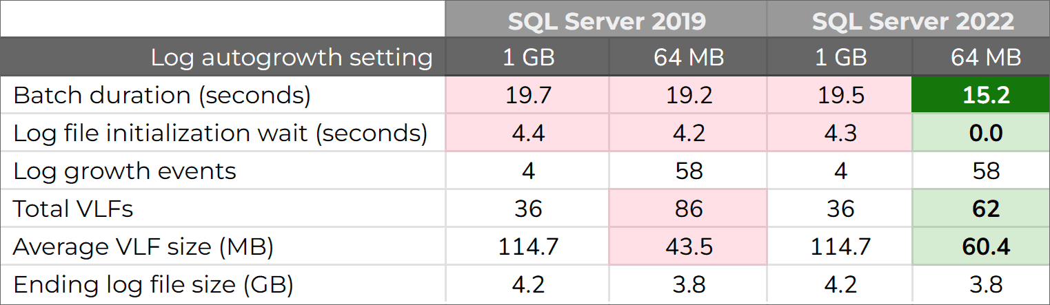
Those are favorable and promising results – we’re shaving roughly 20% off the workload duration simply by moving to 64 MB autogrowth, entirely due to eliminating PREEMPTIVE_OS_WRITEFILEGATHER waits and capitalizing on instant file initialization. In addition, we see a slight benefit from an improved VLF algorithm (recently documented), resulting in fewer, larger VLFs for the exact same log growth events.

Now, your mileage may vary. On more capable hardware, the percentage of time spent on initialization may be lower, so the benefit might be more subtle. Still, zeroing out a new portion of a log file will never be instantaneous for growth events larger than 64 MB (barring more enhancements in future versions, of course). So, as you start planning for SQL Server 2022, or even if you’re already there, this configuration option is worth testing against your workload and hardware. This is especially true if you’re not in a position to pre-size your log files bigger than you’ll ever need. After all, the fastest file change is the one that doesn’t have to happen in the first place; the next fastest is the one that can take advantage of instant file initialization.

The post Changing log growth strategy in SQL Server 2022 appeared first on Simple Talk.


from Simple Talk https://ift.tt/Wd3TGIk
via

Friday, May 12, 2023

Uncovering the mysteries of PostgreSQL (auto) vacuum

Welcome to the second blog of the “magic of parameters” series. In the first entry, I covered memory parameters, and in this article. In this article will talk about PostgreSQL configuration parameters which manage the (auto)vacuum and (auto)analyze background processes.

Why vacuuming is necessary?

Before we start talking about vacuum and analyze-related parameters, we need to touch on the concept of vacuuming in PostgreSQL. This concept is Postgres-specific, and for DBAs coming from Oracle and Microsoft SQL Server it might feel confusing – you can’t directly map it to any previous experiences. (Note: both Oracle SQL Server do share some similarities in some of their configurations. For example, SQL Server memory optimized tables have a similar process referred to as garbage collection.)

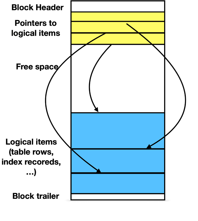
Let’s start by looking at how data is stored in PostgreSQL database. The generic structure of a block is shown in Figure 1.

Figure 1. Generic block structure

Table rows are stored in a heap, and their order is not guaranteed. In Figure 1, you can see free space in the block, which can be filled with new rows of data. If your previous DBA experience is with a lock-based RDBMS engine, you would think that we should set up a fillfactor less than 100% for each table so that there will be some room to maintain most updated records in the same block.

Be ready for a surprise! Although you can define a fillfactor <100%, this option is rarely used in PostgreSQL. The reason is that PostgreSQL never updates a row in place due to how it implements concurrency controls!

Multi-version concurrency control

To allow multiple users to access data concurrently and to avoid waits when data is being updated, PostgreSQL uses multi-version concurrency control (MVCC). It is implemented using Snapshot Isolation (SI): each SQL statement sees a snapshot of data (a database version) as it was when the transaction started, regardless of the current state of the underlying data. This approach provides multiple advantages:

  • It prevents statements from viewing inconsistent data due to table modifications made by other transactions
  • It provides transaction isolation for each session

The modified tuples are saved in a new place, within the same block or in a different block, but if some transactions still are still actively accessing the old versions of the modified tuples, these tuples are kept “alive.”

How does Postgres know which versions should be kept alive, and which can be recycled? Each table has several “hidden” (system) attributes which you can’t see when you execute SELECT * FROM <table>. Two of these hidden attributes are xmin, which contains the ID of the transaction which created the row, and xmax, stores the ID of the transaction which deleted the row (either by updating or by deleting).

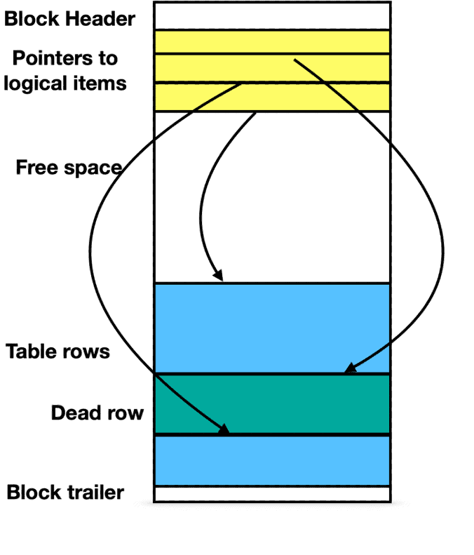
Now, for any processes transaction ID that is between greater or equal to xmin and less than xmax, this row is active and should be visible to that transaction. PostgreSQL marks a tuple dead if there are no more active transactions that the row could be visible to. Figure 2 presents a block layout with a dead tuple.

Shape Description automatically generated with medium confidence

Figure 2. Block layout with dead tuple.

What is the effect of MVCC on the database performance? On the one hand, the absence of locking facilitates performance. On the other hand, having multiple versions and thereby dead tuples creates both table and index bloat.

What’s VACUUM for?

VACUUM checks all the blocks and marks the old tuples “dead.” It’s important to remember that VACUUM does not rewrite the block and does not “compress” the data. It simply marks the space occupied by dead tuples as “reusable.” You can compress data and return the unused space back to the operating system by running VACUUM FULL.

What else does VACUUM do?

By this time, it might already feel like “too much information”, especially if that’s the first time you are exposed to the concept of vacuuming in Postgres. But before we proceed further, let’s note that the job of VACUUM is not limited to reclaiming space. In addition, it:

  • Updates data statistics used by the PostgreSQL query planner.
  • Updates the visibility map, marking the blocks with no dead tuples
  • Protects against loss of very old data due to transaction ID wraparound.

If your job is to manage Postgres instances, you might want to do more reading on the topic of vacuuming, beyond what we will cover, but for the start, let’s just keep in mind there are many things vacuum does.

What’s Autovacuum for?

Autovacuum is a daemon which periodically invokes vacuuming of tables and indexes. Autovacuum does not require any scheduling, instead, its behavior is driven by several system parameters, which will be described later in this article.

Myths about the vacuuming process

Since the concept of vacuuming is not as common in other RDBMS and is not all that we;; understood by PostgreSQL newbies (and some experienced people too!), it is a source for multiple common myths.

In this section I will do what I can to dispel these myths.

Myth #1. The vacuum process makes everything run slower

The reality. VACUUM (and by extension, autovacuum) is obviously not cost-free, but the cost is far less than if it was not executed. When rows are being modified, dead tuples begin to accumulate and everything can become slow when the autovacuum does not run regularly.

Tables become bloated (more details on table bloat later in the article), which makes sequential scans slower. Visibility map is not updated, which prevents the usage of index-only scan (PostgreSQL still needs to check the heap to make sure that index does not point to any dead tuples).

Myth #2. The vacuum process blocks other operations

The reality. The VACUUM process is aborted if it is blocking any write operation. The wait time is determined by the deadlock_timeout parameter. In fact, on a busy table, it may be beneficial to run vacuum often (ideally using autovacuum), because otherwise, it might not have a chance to finish for days and weeks, because it is blocked by write operations.

Myth #3. On busy mission-critical databases, it’s a good idea to disable autovacuum and run scheduled vacuum jobs during the quiet time.

The reality. “Busy systems” (in terms of modifying data) may be busy most of the day, not just certain times of the day, with very few exceptions. If you disable autovacuum and run vacuum on a schedule, such as during “quiet time,” vacuum will end up with more job to do (if the system is “busy” there could easily be a lot of dead tuples by that time!). Now, you might end up blocking the tables for longer periods of time, so you need to make sure that there are no write operations for the extended period of time.

In addition, even if the system behavior is predictable in general, there are chance of burst updates, and you may end up with more bloat than expected, with even more severe consequences.

Myth #4. If you use other ways to control bloat, like pg_squeeze, you do not need to run vacuum at all.

The reality. Recall that reclaiming the space is only one of several functions performed by VACUUM. You might be able to reclaim the space, but other vacuum functions won’t be performed, most importantly, old records won’t be frozen. Once again if we are talking about “busy systems” the risk of TXID wraparound is higher.

Myth #5. You need to monitor the autovacuum runs and make sure that all tables are vacuumed at least daily

The reality. On the tables with few writes autovacuum might run once a week or even less frequent. The parameters explained in the next section determine how often vacuuming will be performed on specific tables.

It is possible to view the statistics on updates for each table and to set up some monitoring based on this information, but that would effectively mean replicating the logic of autovacuum. More important is to monitor system performance and tables bloat

The most important parameters that govern the vacuum process

There are many vacuum-related parameters which allow very precise vacuum tuning. However, in practice, it is often enough to set up correctly just a handful of them. Most of them control autovacuum, to help tune the automatic execution of the vacuum process.

  • autovacuum_vacuum_cost_delay: amount of time the process will sleep after the max cost exceeded
    • The default value is 20 ms, which is very conservative and may result in vacuuming not keeping up with changes. Start with reducing it to 10ms, and if necessary, you can go as low as 2 ms.
    • Note that this parameter is different from the naptime (see below)
  • autovacuum_max_workers: max parallel workers (across server) which are invoked for each autovacuum invocation.
    • Most often, this parameter is set to half of the total number of parallel workers defined for the instance, however, it is often beneficial to increase this number even more.
  • autovacuum_naptime: minimum delay between autovacuum runs on any given database.
    • Each time the autovacuum daemon starts, it examines the database and issues VACUUM and ANALYZE commands as needed for tables in that database. Since this setting determines the wake-up time per database, an autovacuum worker process will begin as frequently as autovacuum_naptime / number of databases. For example, if autovacuum_naptime = 1 min and we have five databases, an autovacuum worker process would be started every twenty seconds.
    • The default value for this parameter is 1 min, however, on busy databases with many writes it can be beneficial to increase its value to prevent autovacuum waking up too often. With this parameter, like with many others, there is a trade-off between “too often” and “too much work on each invocation”.
  • autovacuum_vacuum_scale_factor: percentage of changes to the table after which a vacuum should run
    • The default value for this parameter is 0.2; for larger tables, should be reduced to 0.05 (and consider this for all tables for that matter)
  • autovacuum_analyze_scale_factor: percentage of changes to the table after which an analyze should run
    The default value is 0.1; for larger tables, should be reduced to 0.05 (and consider for all tables here as well) respectively.
    • Note: The default for the autovacuum_vacuum_scale_factor is 0.2 (20%) and autovacuum_analyze_scale_factor is 0.1 (10%). While the default values perform acceptably for tables of a modest size (up to around 500MB), for larger tables these values are usually too high.
  • autovacuum_vacuum_cost_limit: The default value of -1 for autovacuum_vacuum_cost_limit results in autovacuum_vacuum_cost_limit = vacuum_cost_limit. However, this value is distributed proportionally among the running autovacuum workers. This is done in order that the sum of the limits of each worker never exceeds the limit on this variable. Therefore, the default value of 200 for vacuum_cost_limit is generally too low for a busy database server with multiple autovacuum workers.should be set to -1
  • vacuum_cost_limit: cumulative cost after which the vacuum should stop, should be set to 200 X number of workers

How to tune (auto)vacuum

Vacuuming is vital for PostgreSQL databases well-being, and autovacuum should never be turned off unless there are really exceptional and unusual circumstances. At the same time, autovacuum should be always tuned for specific environment needs.

Tuning autovacuum is challenging, because we need to take into account the vacuuming speed, level of I/O, and blocking. To start with, the default set of vacuum-related parameters would work adequately. After some time passes, check system bloat and if it appears to be high and adjust the autovacuum settings. What should be considered a high bloat depends on many factors.

On average, bloat below 20% is considered normal. For larger tables, 10% maybe considered a significant bloat, while for small tables, even 50% bloat maybe fine. If the bloat does not result in visible performance degradation, there is no pressing need to address it.

How to determine if your tables are bloated

There are examples of such queries that can be found in many PostgreSQL blogs and company’s websites. Many of the solutions require extensions, if you are up to installing additional extensions to monitor your bloat, you can use the following:

CREATE EXTENSION pgstattuple;

This is one of many extensions provided with PostgreSQL contrib package, so you do not need to download anything, just execute the CREATE statement. The available functions are documented in PostgreSQL documentation.

If you do not want to install any extensions, the following queries will provide good estimates:

table_bloat_check.sql

index_bloat_check.sql

If your system is even somewhat active, it is essential that you monitor the bloat in your data objects.

How to monitor

Although you can find the last time when vacuum/autovacuum and analyze/autoanalyze were executed in the pg_stat_all_tables, we do not recommend monitoring this value. As it was mentioned in the previous section, if the updates didn’t reach a threshold, the is no need for autovacuum to run. However, the pg_stat_all_tables object contains a lot of valuable information which may be very useful for evaluating the database health.

For each table, pg_stat_all_tables contains the following information:

Column

Description

seq_scan

Number of sequential scans on the table

seq_tup_read

Number of tuples read using sequential scan

idx_scan

Number of index scan accesses to the table

idx_tup_fetch

Number of tuples fetched using index scan

n_tup_ins

Number of tuples inserted

n_tup_upd

Number of tuples updated

n_tup_hot_upd

Number of “hot updates” (updates which keep the tuple in the same block)

n_live_tup

Estimated number of live tuples in the table

n_dead_tuples

Estimated number of dead tuples in the table

n_mod_since_analyze

Estimated number of modifications since last analayze

n_ins_since_vacuum 

Estimated number of inserts since last vacuum

last_vacuum

Time of the last vacuum run on that table

last_autovacuum

Time of the last autovacuum run on that table

last_analyze

Time of the last analyze run on this table

last_autoanalyze

Time of the last autoanalyze run on that table

vacuum_count

Total number of vacuum runs on the table

auto_vacuum_count

Total number of autovacuum runs on the table

analyze_count

Total number of analyze runs on the table

autoanalyze_count

Total number of autoanalyze runs on the table

As you can see, this table provides valuable information about the dynamics of each table. However, the only way to see whether the autovacuum is tuned correctly is to run bloat checking queries on regular basis.

Conclusion

It is not uncommon that new PostgreSQL users and even DBAs do not pay much attention to tuning autovacuum and monitoring tables and indexes bloat. This happens since these concepts are Postgres-specific and are not in the mental checklist of database professionals with previous experience elsewhere.

Thereby, it is important to educate yourself about the role vacuum and analyze play in the PostgreSQL databases well-being.


The post Uncovering the mysteries of PostgreSQL (auto) vacuum appeared first on Simple Talk.


from Simple Talk https://ift.tt/hWUXgHw
via

Tuesday, May 9, 2023

Xerox stars for accessibility

I was working for Xerox when the Xerox Star, precursor to all the computer systems in use today, was introduced. Before then, computer users just had command-line or character-based GUIs. The Xerox Star workstations were displayed for the first time for us insiders in a special room, like a secular chapel, guarded over by the priesthood of developers. We were amazed. Many of the ideas had been around, but never combined into a complete graphical system. What were we amazed by? The Graphics? No. The proportional fonts? No. For common usage, this was, at the time, in the science-fiction realm of affordability. It was the accessibility that amazed us.

In the narrowest sense, the windowing system that Palo Alto designed allowed people with disabilities such as poor sight, hearing or motor control to have comparable opportunities to access computing resources. Applications could be configured to provide alternative ways of using their features with different visual clues, without mouse or bypassing the keyboard. Each application had the same style, layout, and menu system, so that you had a good chance of finding yourself around an application well enough to start using it, even the very first time you tried. Folks with perceptual access deficits fared well because any icons were used only in addition to the menus and had accompanying text or ‘mouse-overs’. There were rules for background and foreground colours, text size and do on. A huge amount of work went on in the ensuing years into finding the optimal rules to make the user interface accessible to people of any language, culture, age, or disability.

For many years everyone mostly stuck to the rules. I’ve developed applications that were designed to comply with a corporate usability manual and had to be signed off by teams of usability experts, user representatives and even the unions, and very right too. They were to be used by people for their entire working day, for maybe years and there was a huge productivity payoff for getting everything right. We used ‘usability testing’ where people unfamiliar with our system were asked to perform simple tasks whilst we, in another room behind a two-way mirror, groaned at our simple design mistakes.

Now, pretty much anything goes. I recently came across a black search box with a black background, for example; Microsoft ditched the Xerox Star menu system for its office products in favour of the ‘office ribbon’; Those who stick to the rules for accessibility are made to seem staid, dull and old-fashioned. The rule-breakers look cool and also lock their users in because of the learning required for change. Maybe it is time to fight back.


The post Xerox stars for accessibility appeared first on Simple Talk.


from Simple Talk https://ift.tt/wdH7Pep
via

Friday, May 5, 2023

Importing data into a MySQL database using LOAD DATA

Database and development teams often load data from plain text files into their MySQL databases. The files might be used to add lookup data, support test and development environments, populate new MySQL instances, load data from regular feeds, or in other ways support their operations. To help with the import process, MySQL provides the LOAD DATA statement, which reads rows from a text file and inserts them into the target table.

In this article, I show how to use the LOAD DATA statement to add data from comma-separated values (CSV) files and other plain text files. Although the examples are fairly basic, they demonstrate the fundamental components that go into a LOAD DATA statement and some of the issues you might run up against along the way. Each example retrieves data from a file on the local system and adds the data to the manufacturers table in the travel database, which you’ve seen in previous articles in this series.

Note: The examples in this article are based on a local instance of MySQL that hosts a very simple database and table. The last section of the article—“Appendix: Preparing your MySQL environment”—provides information about how I set up my system and includes a SQL script for creating the database and table on which the examples are based.

Connecting to the MySQL server

Importing data from a text file into a MySQL database is in itself a fairly straightforward process. Often the most difficult part of the operation is setting up your environment to ensure that it will allow you to run a LOAD DATA statement and import the data into the target table. As with any SQL statement in MySQL, you must have been granted the privileges necessary to carry out your operations (a topic beyond the scope of this article). However, there are a few other issues to be aware of in order to import data, starting with the LOCAL option.

When you create a LOAD DATA statement, you can include the LOCAL option as part of the statement definition. The option determines the statement’s security requirements as well as whether the source text file is located on the client system or the server hosting the MySQL instance:

  • If you do not specify the LOCAL option, the source text file must be located on the MySQL host. When you run the LOAD DATA statement, MySQL reads the file directly from the directory and inserts the data into the target table. This approach generally performs a little better than when you include the LOCAL option because the data is loaded more directly. However, getting the connection right is much more difficult (and the topic for many online discussions).
  • If you specify the LOCAL option, the source text file must be located on the client machine. The client reads the file and sends the content to the server, where it is stored in a temporary file until it is loaded into the target table for processing. The LOCAL option also works if the client and MySQL are on the same machine, which is the approach I’ve taken for this article. Connectivity is typically much easier to establish when you use the LOCAL option.

For the examples in this article, I have used the LOCAL option. Not only are the MySQL connectivity requirements more complicated without it, but they are also not well documented, adding to the frustration should you run into any glitches. If you check out the various forum postings that discuss connectivity issues around the LOAD DATA statement, you’ll find that in many cases, people responding to a post suggest the use of the LOCAL option as a simple workaround to the various challenges.

I also think that for many database administrators and developers, locating source files on the client side is preferable to uploading those files to the MySQL server, if they’re even permitted to do so. If you use the LOCAL option, you do not need the FILE privilege to run a LOAD DATA statement, and you can store the source text file in any local folder that can be accessed by the client application, which in this case, is MySQL Workbench.

Note: The MySQL documentation states that “if LOCAL is specified, the file must be located on the client host.” However, I was able to run a LOAD DATA statement that included the LOCAL option and that pulled data from other systems on my network. The first was another Mac computer and the other was Windows 11 virtual machine. I have not tested this capability beyond that.

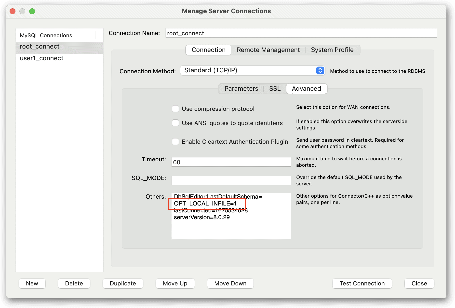
When using the LOCAL option, you must ensure that data-loading is enabled on both the client side and server side. To enable it on the client side in Workbench, you should modify your connection on the tool’s home screen. In the main window, right-click the connection and click Edit connection. On the Connection page of the Manage Server Connections dialog box, select the Advanced tab and add the following command in the Others box:

OPT_LOCAL_INFILE=1

The command sets the local-infile option to ON, making it possible to run a LOAD DATA statement that includes the LOCAL option. The following figure shows the setting (outlined in red) as it appears on the connection’s Advanced tab. This setting applies only to this user’s connections in Workbench. Other connections must be configured individually.

In addition to enabling the local-infile option, you must also enable the local_infile global variable on the server, if it’s not already enabled. (The only difference between these two names is that the global variable uses an underscore rather than a dash.) To confirm the variable’s setting, you can run a SHOW GLOBAL VARIABLES statement against your MySQL instance:

SHOW GLOBAL VARIABLES LIKE 'local_infile';

If the statement returns a value of ON, then you’re all set. If the statement returns OFF, then you should run the following SET statement to enable the variable:

SET GLOBAL local_infile = 1;

Once you’ve enabled local data-loading on both the client and server, you should be ready to run your LOAD DATA statements. The examples that follow demonstrate different aspects of importing data from a text file. I’ll show you the contents of each file as we work through the examples. You can then create them on your own system if you want to try out the examples for yourself.

Introducing the LOAD DATA statement

Before we get into the first example, it’s important to understand the basic components that go into a LOAD DATA statement, which includes a number of clauses and subclauses. The following syntax simplifies the statement somewhat to give you an overview of the statement’s essential elements and how they fit together:

LOAD DATA [LOCAL] 
INFILE 'file_name'
[REPLACE | IGNORE]
INTO TABLE table_name
FIELDS
  [TERMINATED BY 'string']
  [[OPTIONALLY] ENCLOSED BY 'char']
  [ESCAPED BY 'char']
LINES
  [STARTING BY 'string']
  [TERMINATED BY 'string']
IGNORE n LINES
[(column_list)]

The LOAD DATA clause is where you specify whether to include the LOCAL option. As I mentioned earlier, this is the approach I’ve taken in this article. The next clause, INFILE, specifies the path and filename (in quotes) of the source text file. You can provide an absolute path or relative path. If relative, the path is relative to the invocation directory.

You can then specify either REPLACE or IGNORE, which are both optional. The REPLACE option tells MySQL to replace existing rows that have the same unique key value. The IGNORE option tells MySQL to ignore rows with the same key value. The IGNORE option has the same effect as the LOCAL option, so if you’re using LOCAL, you never need to use IGNORE. However, you can use the REPLACE option with LOCAL.

The INTO TABLE clause specifies the name of the target table. The main thing here is to be sure that you’ve been granted the privileges necessary to add data to that table.

The FIELDS clause comes next, and it supports one or more of the following three subclauses:

  • The TERMINATED BY subclause specifies the string used in the text file to terminate each field. The string can be one or more characters. The default value is \t for tab, which means that tabs are used to separate field values.
  • The ENCLOSED BY subclause specifies the character used in the text file to enclose values, such as quotation marks around string values. The OPTIONALLY keyword, which itself is optional, is used “if the input values are not necessarily enclosed within quotation marks,” according to MySQL documentation. (More on that in a bit.) The default value for the ENCLOSED BY subclause is an empty string, indicating that the fields are not enclosed in quoting characters.
  • The ESCAPED BY subclause specifies the character used in the text file for escaping characters that could impact how MySQL interprets the data. The default value is a backslash (\), which is also used in MySQL to escape characters, including the backslash itself. Many programming languages also use the backslash to escape characters.

The FIELDS clause is itself optional, but if you include it, you must specify at least one of the subclauses.

Note: The OPTIONALLY option in the ENCLOSED BY subclause is one of the most confusing elements in the LOAD DATA statement. Its use made no difference in the various tests I ran. For example, in one test, I enclosed all the values in the manufacturer fields in double quotation marks except for one. MySQL imported the data correctly whether or not I included the OPTIONALLY option. I also tested the option using NULL values and empty strings and received the same results. There might be use cases in which the option does make a difference, but I have yet to discover them. However, the FIELDS and LINES clauses in the LOAD DATA statement are the same as the SELECT…INTO OUTFILE statement, and much of the discussion in the MySQL documentation about the OPTIONALLY option is related to SELECT…INTO OUTFILE, so perhaps that is where it is most relevant.

Like the FIELDS clause, the LINES clause is also optional. The LINES clause supports the following two subclauses:

  • The STARTING BY clause specifies the common prefix used at the beginning of each line in the text file. The default value is an empty string, indicating that no specific prefix is used. If a prefix is specified and a line does not contain that prefix, MySQL skips the line when importing the data.
  • The TERMINATED BY clause specifies the string used in the text file to terminate each line. The string can be one or more characters. The default value is \n, which refers to a newline character (linefeed). I created my text file in Apple’s TextEdit app, so the default worked on my system, but not all systems operate the same. For example, if you create the text files in Windows, you might need to specify '\r\n' as the TERMINATED BY value.

If you include both the FIELDS clause and LINES clause, the FIELDS clause must come first. The IGNORE n LINES clause comes after these two clauses. The IGNORE n LINES clause specifies the number of lines to skip at the beginning of the file when importing the data. The clause is commonly used when the file contains a header row, in which case, the clause would be written as IGNORE 1 LINES.

The final clause is the list of columns, which are enclosed in parentheses and separated by commas. Although this clause is optional, you will likely include it in most of your statements, unless you’re source data contains a field for every column and the fields are in the same order as the columns.

The LOAD DATA statement contains a few other clauses, but the ones I’ve shown you here are plenty for you to get started. Even so, I recommend that you review the MySQL topic LOAD DATA Statement to learn more about the statement’s various elements.

Importing a CSV file

Now that you’ve been introduced to the LOAD DATA statement, let’s look at some examples that show it in action. You can refer back to the previous section if needed as you work through the following sections.

In preparation for the first example, I created a file named manufacturers1.csv and added the following data:

101,Airbus
102,Beagle Aircraft Limited
103,Beechcraft
104,Boeing
105,Bombardier
106,Cessna
107,Embraer

I saved the file to the folder /Users/mac3/Documents/TravelData/ on my local computer. If you plan to try out the examples for yourself, you can save the files to any location on your system that Workbench can access. Just be sure to update the file path in the examples before you run your statements.

After I created the manufacturers1.csv file, I ran the following LOAD DATA statement, which saves the data to the manufacturers table in the travel database:

LOAD DATA LOCAL INFILE 
  '/Users/mac3/Documents/TravelData/manufacturers1.csv' 
INTO TABLE manufacturers 
FIELDS TERMINATED BY ',' 
(manufacturer_id, manufacturer);

As you can see, the LOAD DATA clause includes the LOCAL option, and the INFILE clause specifies the source file. These are followed by the INTO TABLE clause, which points to the manufacturers table.

The next clause, FIELDS, includes the TERMINATED BY subclause, which specifies that a comma is used as the field separator, rather than the default tab. The statement then provides the names of the two target columns—manufacturer_id and manufacturer—which are enclosed in parentheses.

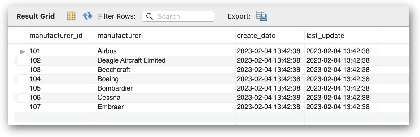
When you run the statement, MySQL extracts the data from the file and populates the manufacturers table. You can verify that the data has been added to the table by running the following SELECT statement:

SELECT * FROM manufacturers;

The SELECT statement returns the results shown in the following figure, which indicates that the data was successfully inserted into the table. Keep this statement handy because you can use it to verify your results for the remaining examples.

To keep things simple for this article, you can also run the following TRUNCATE statement to remove the data from the manufacturers table in preparation for the next example:

TRUNCATE TABLE manufacturers;

You should keep this statement handy as well. You’ll want to run it after most of the following examples, except in a couple instances where I demonstrate specific concepts, in which case, I’ll let you know not to run it.

Ignoring the first lines in an import file

Some of the source files that you work with might contain a header row that lists the field names or include other types of information, such as comments about when and where the file was generated. You can skip these rows when importing the data by including the IGNORE n LINES clause in your LOAD DATA statement.

To see how this works, create a text file named manufacturers2.csv file, add the following data to the file, and save it to the same location as the manufacturers1.csv file:

manufacturer_id,manufacturer
101,Airbus
102,Beagle Aircraft Limited
103,Beechcraft
104,Boeing
105,Bombardier
106,Cessna
107,Embraer

Now run the following LOAD DATA statement, which includes an IGNORE 1 LINES clause that tells MySQL to skip the first row:

LOAD DATA LOCAL INFILE 
  '/Users/mac3/Documents/TravelData/manufacturers2.csv' 
INTO TABLE manufacturers 
FIELDS TERMINATED BY ',' 
IGNORE 1 LINES
(manufacturer_id, manufacturer);

After you execute the LOAD DATA statement, you can again run your SELECT statement to verify that the correct data has been added. The results should indicate that the header row has been omitted. You can then run your TRUNCATE statement again in preparation for the next example.

The IGNORE n LINES clause is not limited to one row. For instance, the following IGNORE n LINES clause specifies five rows rather than one:

LOAD DATA LOCAL INFILE 
  '/Users/mac3/Documents/TravelData/manufacturers2.csv' 
INTO TABLE manufacturers 
FIELDS TERMINATED BY ',' 
IGNORE 5 LINES
(manufacturer_id, manufacturer);

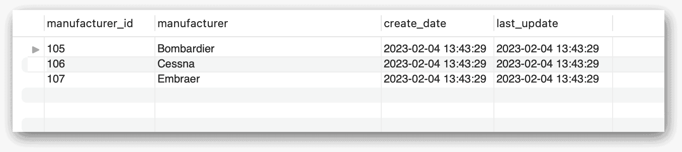
When you run the SELECT statement this time, you should get the results shown in the following figure. (Don’t truncate the table for this example or the next one because I want to point out of a couple other issues.)

As you can see, the table contains only the last three rows from the source file. However, suppose that you were to run the statement again, only this time, specifying only one row in the IGNORE n LINES clause:

LOAD DATA LOCAL INFILE 
  '/Users/mac3/Documents/TravelData/manufacturers2.csv' 
INTO TABLE manufacturers 
FIELDS TERMINATED BY ',' 
IGNORE 1 LINES
(manufacturer_id, manufacturer);

When you execute the statement, MySQL tries to insert all seven rows of data into the target table, but only the first four rows succeed. After running the statement, MySQL returns the following message:

4 row(s) affected, 3 warning(s): 1062 Duplicate entry '105' for key 'manufacturers.PRIMARY' 1062 Duplicate entry '106' for key 'manufacturers.PRIMARY' 1062 Duplicate entry '107' for key 'manufacturers.PRIMARY' Records: 7 Deleted: 0 Skipped: 3 Warnings: 3

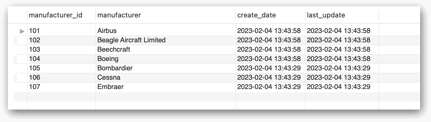
The message indicates that the existing rows with manufacturer_id values of 105, 106, and 107 were skipped. That is, no new rows with these values were inserted into the table. Only the first four rows were added. If you run the SELECT statement again, you should receive results similar to those shown in the following figure. (Once again, don’t truncate the table; leave it for the next example.)

The table now contains all seven rows of data, but if you look closely at the timestamps in the figure, you’ll see that the last three rows precede the first five rows by nearly 30 seconds. (I ran the last two LOAD DATA statements fairly close together.)

Now suppose you run the same LOAD DATA statement again, only this time you include the REPLACE option:

LOAD DATA LOCAL INFILE 
  '/Users/mac3/Documents/TravelData/manufacturers2.csv' 
REPLACE
INTO TABLE manufacturers 
FIELDS TERMINATED BY ',' 
IGNORE 1 LINES
(manufacturer_id, manufacturer);

When you execute the statement, MySQL now returns the following message:

14 row(s) affected Records: 7 Deleted: 7 Skipped: 0 Warnings: 0

The message indicates that 14 rows were processed. However, only seven records were affected, and seven were deleted. This means that the database engine deleted the seven existing records and re-added them to the table. You can verify this be running the SELECT statement again. Your results should show different timestamps than in the previous results, with the all values very close, if not the same.

You can now rerun your TRUNCATE TABLE statement to prepare the manufacturers table for the next example.

Working with quoted fields in the import file

When importing data, your text files might include some or all fields enclosed in quotation marks. For example, I created the manufacturers3.csv file using the following data, which includes single quotation marks around the string values:

manufacturer_id,manufacturer
101,'Airbus'
102,'Beagle Aircraft Limited'
103,'Beechcraft'
104,'Boeing'
105,'Bombardier'
106,'Cessna'
107,'Embraer'

To handle the quoted fields, you can add an ENCLOSED BY subclause to your FIELDS clause, as shown in the following example:

LOAD DATA LOCAL INFILE 
  '/Users/mac3/Documents/TravelData/manufacturers3.csv' 
INTO TABLE manufacturers 
FIELDS TERMINATED BY ',' ENCLOSED BY '\''
IGNORE 1 LINES
(manufacturer_id, manufacturer);

The ENCLOSED BY subclause specifies that a single quotation mark is used to enclose fields. The quotation mark is preceded by a backslash to escape the character when submitting it to the database engine. If you don’t use the ENCLOSED BY subclause, the database engine will treat the quotation marks as literal values and store them along with the rest of the values.

After you execute the LOAD DATA statement, you can run your SELECT statement to verify the results and then run your TRUNCATE statement to prepare the manufacturers table for the next example.

When you specify a single quotation mark in the ENCLOSED BY subclause, you can enclose it in double quotes, rather than escaping it with a backslash:

LOAD DATA LOCAL INFILE 
  '/Users/mac3/Documents/TravelData/manufacturers3.csv' 
INTO TABLE manufacturers 
FIELDS TERMINATED BY ',' ENCLOSED BY "'"
IGNORE 1 LINES
(manufacturer_id, manufacturer);

In some cases, the text file will use double quotation marks to enclose field values, rather than single quotation marks. To demonstrate how to handle these, I created the manufacturers4.csv file using the following data:

manufacturer_id,manufacturer
101,"Airbus"
102,"Beagle Aircraft Limited"
103,"Beechcraft"
104,"Boeing"
105,"Bombardier"
106,"Cessna"
107,"Embraer"

To handle this file, the ENCLOSED BY subclause should be modified to specify a double quotation mark, enclosing it in single quotation marks:

LOAD DATA LOCAL INFILE 
  '/Users/mac3/Documents/TravelData/manufacturers4.csv' 
INTO TABLE manufacturers 
FIELDS TERMINATED BY ',' ENCLOSED BY '"'
IGNORE 1 LINES
(manufacturer_id, manufacturer);

After you run this LOAD DATA statement, you can once again run your SELECT statement to verify the results. Once you’ve reviewed them, you can then run your TRUNCATE statement in preparation for the next example. (You should do this for all the remaining examples.)

Working with different formats in your text files

The text files that you work with might be table-delimited rather than comma-delimited, and they might include other elements that require special handling. Consider the manufacturers5.txt file, which I created with the following data:

manufacturer_id        manufacturer
*,*101  "Airbus"
*,*102  "Beagle Aircraft Limited"
*,*103  "Beechcraft"
*,*104  "Boeing"
*,*105  "Bombardier"
*,*106  "Cessna"
*,*107  "Embraer"

In this case, a tab is used as the field separator, and each line is preceded by the *,* characters. As a result, you don’t need to specify the TERMINATED BY subclause in the FIELDS clause because the tab is the default value, but you do need to take steps to handle the line prefix. For this, you should add a LINES clause with a STARTING BY subclause that specifies the prefix characters:

LOAD DATA LOCAL INFILE 
  '/Users/mac3/Documents/TravelData/manufacturers5.txt' 
INTO TABLE manufacturers 
FIELDS ENCLOSED BY '"'
LINES STARTING BY '*,*'
IGNORE 1 LINES
(manufacturer_id, manufacturer);

When you run this statement, MySQL will use the prefix characters to determine which rows to add, while stripping out the characters in the process.

As already pointed out, the preceding example does not include a TERMINATED BY subclause in the FIELDS clause. It also does not include a TERMINATED BY subclause in the LINES clause because the text file uses the default linefeed value. However, you can still include both clauses if you want:

LOAD DATA LOCAL INFILE 
  '/Users/mac3/Documents/TravelData/manufacturers5.txt' 
INTO TABLE manufacturers 
FIELDS TERMINATED BY '\t' ENCLOSED BY '"'
LINES TERMINATED BY '\n' STARTING BY '*,*'
IGNORE 1 LINES
(manufacturer_id, manufacturer);

When using the STARTING BY subclause, be aware that your text file must use these prefixes consistently or you might get unexpected results. For example, the following text file, manufacturers6.txt, includes a line with two records but no prefix in front of the first record:

manufacturer_id        manufacturer
*,*101  "Airbus"
*,*102  "Beagle Aircraft Limited"
*,*103  "Beechcraft"
104     "Boeing" *,*105 "Bombardier"
*,*106  "Cessna"
*,*107  "Embraer"

After you’ve created the file on your system, you can run the following LOAD DATA statement to see what happens:

LOAD DATA LOCAL INFILE 
  '/Users/mac3/Documents/TravelData/manufacturers6.txt' 
INTO TABLE manufacturers 
FIELDS ENCLOSED BY '"'
LINES STARTING BY '*,*'
IGNORE 1 LINES
(manufacturer_id, manufacturer);

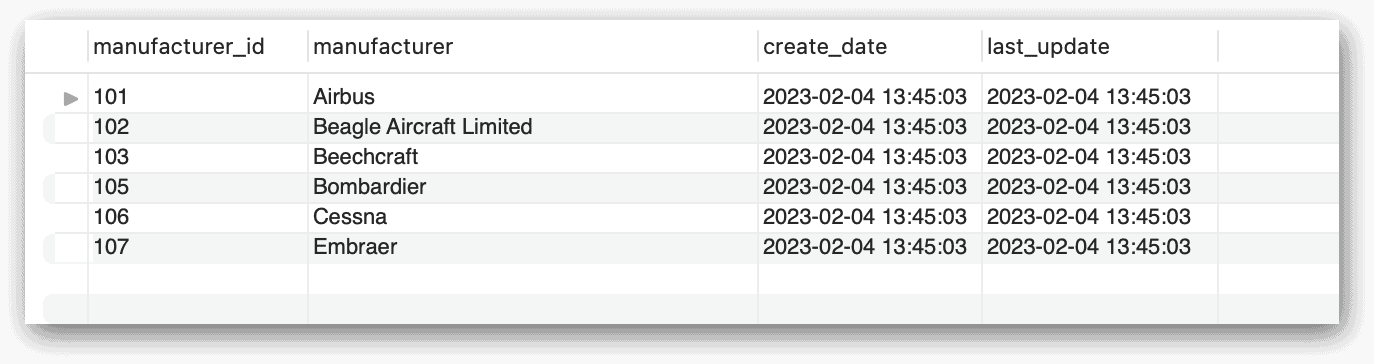
When you execute this statement, MySQL skips the record with a manufacturer_id value of 104 but still adds the record with a value of 105. You can verify this by again running your SELECT statement, which returns the results shown in the following figure.

In some cases, you might run into text files whose lines are terminated with nontraditional characters (as opposed to the usual linefeeds or returns). For example, I created the manufacturers7.txt file using the following data, which separates the lines with triple hash marks (###):

manufacturer_id        manufacturer###101      "Airbus"###102  "Beagle Aircraft Limited"###103 "Beechcraft"###104      "Boeing"###105  "Bombardier"###106      "Cessna"###107  "Embraer"

To accommodate this file, you need to include a TERMINATED BY subclause in your LINES clause that specifies the hashmarks:

LOAD DATA LOCAL INFILE 
  '/Users/mac3/Documents/TravelData/manufacturers7.txt' 
INTO TABLE manufacturers 
FIELDS ENCLOSED BY '"'
LINES TERMINATED BY '###'
IGNORE 1 LINES
(manufacturer_id, manufacturer);

When you run this statement, the database engine will know how to interpret the hashmarks and will insert the data accordingly, stripping out the hashmarks in the process.

In some cases, you might also run into a text file that uses a character other than the backslash to escape characters within fields. For example, the manufacturers8.txt file contains seven lines of comma-delimited fields, one of which includes a comma in the manufacturer name:

manufacturer_id,manufacturer
101,Airbus
102,Beagle Aircraft Limited
103,Beechcraft
104,Aviat Aircraft^, Inc.
105,Bombardier
106,Cessna
107,Embraer

In this case, the name’s comma is escaped with a caret (^). Because this character is not a backslash (the default escape character), you need to add an ESCAPE BY clause that specifies the caret, as shown in the following example:

LOAD DATA LOCAL INFILE 
  '/Users/mac3/Documents/TravelData/manufacturers8.txt' 
INTO TABLE manufacturers 
FIELDS TERMINATED BY ',' ESCAPED BY'^'
IGNORE 1 LINES
(manufacturer_id, manufacturer);

If you do not include the ESCAPE BY clause, the database engine will retain the caret but truncate the manufacturer name, as in Aviat Aircraft^. However, if you include the clause, MySQL will strip out the caret and treat the comma as a literal value, resulting in a column value of Aviat Aircraft, Inc., rather than the truncated version.

Getting started with importing data in MySQL

As mentioned earlier, the LOAD DATA statement includes other elements than what I’ve shown you here. There are also other options for importing data, such as the mysqlimport command-line utility, which generates and sends LOAD DATA statements to the MySQL server. Most of the utility’s options correlate directly to the LOAD DATA statement. Another option is the Table Data Import wizard in MySQL Workbench. The wizard walks you through the process of importing data from a CSV or JSON file.

If you work with MySQL databases on a regular bases, chances are good that you’ll want to import data from text files, even if only to set up test or development environments. In most cases, what I’ve shown you here will be enough to get you started with the LOAD DATA statement. Just know that that you might run into situations that I haven’t covered, in which case, it’s always a good idea to review other MySQL documentation to help you fill in the gaps.

Appendix: Preparing your MySQL environment

When creating the examples for this article, I used a Mac computer that was set up with a local instance of MySQL 8.0.29 (Community Server edition). I also used MySQL Workbench to interface with MySQL. The examples import data from a set of sample text files that I created in Apple’s text editor, TextEdit.

I provide you with the files’ contents throughout the article, along with the example LOAD DATA statements. If you plan to try out these examples, you can create the files on your own system as you work through those examples. Before you get started, however, you should run the following script against your MySQL instance:

DROP DATABASE IF EXISTS travel;

CREATE DATABASE travel;
USE travel;
CREATE TABLE manufacturers (
  manufacturer_id INT UNSIGNED NOT NULL,
  manufacturer VARCHAR(50) NOT NULL,
  create_date TIMESTAMP NOT NULL DEFAULT CURRENT_TIMESTAMP,
  last_update TIMESTAMP NOT NULL 
    DEFAULT CURRENT_TIMESTAMP ON UPDATE CURRENT_TIMESTAMP,
  PRIMARY KEY (manufacturer_id) );

The script creates the travel database and adds the manufacturers table. Otherwise, that’s all you need for the try out the examples (in addition to creating the source text files). For most of the examples, I simply truncated the data to prepare the table for the next example. If you already created the database and table for previous articles, I recommend that you re-create them now or at least truncate the manufacturers table before getting started.


The post Importing data into a MySQL database using LOAD DATA appeared first on Simple Talk.


from Simple Talk https://ift.tt/jGM42Nz
via

Monday, May 1, 2023

PostgreSQL Basics: Essential psql Tips and Tricks

Having access to the psql command-line tool is essential for any developers or DBAs that are actively working with and connecting to PostgreSQL databases. In our first article, we discussed the brief history of psql and demonstrated how to install it on your platform of choice and connect to a PostgreSQL database.

In this article we’ll get you up and running with all of the essential things you need to know to start on your journey to becoming a psql power-user. From basic command syntax to the most common (and helpful) meta-commands, it’s all covered throughout the rest of the article.

To get the most value out of this content, you should have psql installed and connected to a PostgreSQL database so that you can try the commands as you read.

Essential Usability Tips

The psql utility is packed with many helpful commands to help you explore and manage your database. Any slash command (\) is used to specify a meta-command that will typically run the necessary SQL queries in the background and return the results in a readable format.

First, let’s look at a few tips about how psql works as a command line tool. Knowing how to enable certain features or find help for each meta-command will go a long way in helping you to be a successful user of the tool.

The Semicolon is Required

PostgreSQL adheres to the ANSI SQL standard which specifies the semicolon for statement termination. In psql, you signal the end of a SQL statement by adding the semicolon and pressing enter.

If you don’t add a semicolon, psql will simply provide a new line for you to keep typing as shown below.

pagila_dev=# select * from film
pagila_dev-# ;

The query will not be executed until the semicolon is added.

Command History and Paging

psql is a terminal application and as such it keeps a history of the queries and commands that you have executed. Therefore, you can use the up and down arrows on your keyboard to page through previous commands and statements. This is helpful when you want to run a statement multiple times but change a filter each time.

The history is stored in a file on your local client which means it will be different from computer to computer. You can also configure psql to create a different history file per database or server using the HISTFILE variable in the .psqlrc file.

To see a list of the commands that be been run, use the \s command.

postgres=# \s

\c pagila_
\c pagila_dev
\df
\x
\df
select * from film
;
\s

Autocompletion

psql supports tab-based autocompletion. For many commands, you can use the TAB key to trigger autocompletion or suggestion. If you want to list a table or connect to a different database, begin with the meta-command and then begin to type the object name and press TAB. If there would be more than one match, psql will provide possible matches similar to a Linux terminal.

Expanded Results Table Formatting

One of the first helpful hints I learned early on with psql was that there are two modes for displaying both query and meta-command results. Normally, psql will do the hard work of formatting rows and columns of data in a monospaced font with the right amount of padding for everything to line up – within reason. When terminal wrapping takes place, however, it can be challenging to figure out which data goes with which column.

In these cases, you can print the results in an “expanded” format which is essentially a crosstab of each row showing the column headings on the left and each value on the right. In this format you can page through results one at a time.

You can toggle expanded mode on and off by using the \x command. Below we show a listing of objects in the database, first in the normal table mode and then with expanded mode turned on.

postgres=# \d
                  List of relations
 Schema |          Name           | Type  |  Owner
--------+-------------------------+-------+----------
 public | example_tbl             | table | postgres
 public | pg_stat_statements      | view  | postgres
 public | pg_stat_statements_info | view  | postgres
(3 rows)

postgres=# \x
Expanded display is on.
postgres=# \d
List of relations
-[ RECORD 1 ]-------------------
Schema | public
Name   | example_tbl
Type   | table
Owner  | postgres
-[ RECORD 2 ]-------------------
Schema | public
Name   | pg_stat_statements
Type   | view
Owner  | postgres
-[ RECORD 3 ]-------------------
Schema | public
Name   | pg_stat_statements_info
Type   | view
Owner  | postgres

Quitting the psql Session

Finally, I’d hate for you to feel like you can’t get out of the interactive shell. Any time you want to quit your current psql session, simply use the \q meta-command to get back to your terminal prompt.

postgres=# \q

ryan@redgate-laptop:~$

System Objects and Additional Details

As we review some of the essential commands below you will notice a pattern where many of the commands have multiple forms. Adding a capital S to the end of many commands will include system objects in the output. Also, including a + at the end of the command will return additional details, analogous to a an advanced output mode.

For example, the two commands below both list the tables, views, and sequences of a database, but the second form provides additional details.

postgres=# \d
                  List of relations
 Schema |          Name           | Type  |  Owner
--------+-------------------------+-------+----------
 public | example_tbl             | table | postgres
 public | pg_stat_statements      | view  | postgres
 public | pg_stat_statements_info | view  | postgres
...

postgres=# \d+
                                              List of relations
 Schema |          Name           | Type  |  Owner   | Persistence | Access method |    Size    | Description
--------+-------------------------+-------+----------+-------------+---------------+------------+-------------
 public | example_tbl             | table | postgres | permanent   | heap          | 8192 bytes |
 public | pg_stat_statements      | view  | postgres | permanent   |               | 0 bytes    |
 public | pg_stat_statements_info | view  | postgres | permanent   |               | 0 bytes    |

postgres=# \dS+
                                               List of relations
   Schema   |              Name               | Type  |  Owner   | Persistence | Access method |    Size    | Description
------------+---------------------------------+-------+----------+-------------+---------------+------------+-------------
 pg_catalog | pg_aggregate                    | table | postgres | permanent   | heap          | 56 kB      |
 pg_catalog | pg_am                           | table | postgres | permanent   | heap          | 40 kB      |
 pg_catalog | pg_amop                         | table | postgres | permanent   | heap          | 88 kB      |
 pg_catalog | pg_amproc                       | table | postgres | permanent   | heap          | 72 kB      |
 pg_catalog | pg_attrdef                      | table | postgres | permanent   | heap          | 8192 bytes |
...
 public     | example_tbl                     | table | postgres | permanent   | heap          | 8192 bytes |
 public     | pg_stat_statements              | view  | postgres | permanent   |               | 0 bytes    |
 public     | pg_stat_statements_info         | view  | postgres | permanent   |               | 0 bytes    |


Getting help

Although the output can be overwhelming, you can always view the psql help file that will show you an expansive list of meta-command patterns. Notice that the output is grouped into categories.

postgres=# \?
General
  \copyright             show PostgreSQL usage and distribution terms
  \crosstabview [COLUMNS] execute query and display result in crosstab
  \errverbose            show most recent error message at maximum verbosity
  \g [(OPTIONS)] [FILE]  execute query (and send result to file or |pipe);
                         \g with no arguments is equivalent to a semicolon
  \gdesc                 describe result of query, without executing it
  \gexec                 execute query, then execute each value in its result
  \gset [PREFIX]         execute query and store result in psql variables
  \gx [(OPTIONS)] [FILE] as \g, but forces expanded output mode
  \q                     quit psql
  \watch [SEC]           execute query every SEC seconds

Help
  \? [commands]          show help on backslash commands
  \? options             show help on psql command-line options
  \? variables           show help on special variables
  \h [NAME]              help on syntax of SQL commands, * for all commands

Query Buffer
  \e [FILE] [LINE]       edit the query buffer (or file) with external editor
  \ef [FUNCNAME [LINE]]  edit function definition with external editor
...

Informational
  (options: S = show system objects, + = additional detail)
  \d[S+]                 list tables, views, and sequences
  \d[S+]  NAME           describe table, view, sequence, or index
  \da[S]  [PATTERN]      list aggregates
  \dA[+]  [PATTERN]      list access methods
…

Essential Meta-commands

In my experience with PostgreSQL over the last few years, particularly coming from many years of SQL Server work, learning how to effectively use basic commands in psql has proven to be useful and time saving. Below are the initial set of commands that will help you navigate the PostgreSQL cluster and databases.

There are certainly many more commands than these, but I believe these are the high-level set that you should learn at the outset.

Connecting to a Different Database

The \c command will connect to a new database on the same server. If you connected to the server with the -W switch, then every time you connect to a different database, you will be prompted for the password again, which is almost always a nuisance so I don’t recommend it.

postgres=# \c flywaytest

psql (15.0 (Ubuntu 15.0-1.pgdg20.04+1), server 15.1 (Debian 15.1-1.pgdg110+1))
You are now connected to database "flywaytest" as user "postgres".

flywaytest=#

Notice that the default psql prompt shows the database name of the current connection.

List All Databases

The \l command will list any databases in the current server along with the specified access privileges. Seeing that the database exists in this list does not imply that the current role can connect (\c) to the database. Adding the + will provide additional information including database size.

postgres=# \l+
                                                    List of databases
       Name        |  Owner   | Encoding |  Collate   |   Ctype    | ICU Locale | Locale Provider |   Access privileges
-------------------+----------+----------+------------+------------+------------+-----------------+-----------------------
 advent_of_code    | postgres | UTF8     | en_US.utf8 | en_US.utf8 |            | libc            | postgres=CTc/postgres+
                   |          |          |            |            |            |                 | rptusr=c/postgres
 bulk_example      | postgres | UTF8     | en_US.utf8 | en_US.utf8 |            | libc            |
 flywaytest        | postgres | UTF8     | en_US.utf8 | en_US.utf8 |            | libc            |
 flywaytest_shadow | postgres | UTF8     | en_US.utf8 | en_US.utf8 |            | libc            |

Display Object Details

There are many \d commands in psql. Although most commands aren’t given specific names, most folks in the community refer to this as either the “describe”, “display”, or “details” command. Much like a CLI that allows you to get help for each command by typing something like “help [command]”, psql uses the \d command almost like that.

Most of the \d commands will provide additional details by adding the + to the end. I’ll only show a few examples of that below, but feel free to try it with any of these commands to get more detail.

Display table, view, and sequence objects

The default action for the describe command is to list all tables, views, and sequences in the current database. We showed examples of the detailed output above when discussing the + operator.

postgres=# \d
                  List of relations
 Schema |          Name           | Type  |  Owner
--------+-------------------------+-------+----------
 public | example_tbl             | table | postgres
 public | pg_stat_statements      | view  | postgres
 public | pg_stat_statements_info | view  | postgres

Describe table, view, or sequence details

You can name a specific object to get additional information. Using the + operator will also list constraints and indexes of a table.

postgres=# \d+ example_tbl
                                       Table "public.example_tbl"
 Column |  Type   | Collation | Nullable | Default | Storage  | Compression | Stats target | Description
--------+---------+-----------+----------+---------+----------+-------------+--------------+-------------
 id     | integer |           | not null |         | plain    |             |              |
 notes  | text    |           |          |         | extended |             |              |
Indexes:
    "idx_example_notes" btree (notes)
Access method: heap

Display Specific Object Types

As you might expect, the psql developers provided specific commands for listing individual object types. Adding different letters after the \d command will list only that type of object. All lists support additional detail using the +.

  • E = foreign table (provided by one of many foreign data wrappers)
  • i = indexes
  • m = materialized views
  • s = sequences
  • t = tables
  • v = views
postgres=# \dt

            List of relations
 Schema |    Name     | Type  |  Owner
--------+-------------+-------+----------
 public | example_tbl | table | postgres

Display Roles and Members

Roles are used for connecting to PostgreSQL, assigning database privileges, and specifying object ownership. See our series of posts on PostgreSQL security for more details about Roles.

postgres=# \du
                                        List of roles
 Role name |                         Attributes                         |     Member of
-----------+------------------------------------------------------------+---------------
 dev1      |                                                            | {devgrp}
 dev2      |                                                            | {devgrp}
 devgrp    | Cannot login                                               | {}
 postgres  | Superuser, Create role, Create DB, Replication, Bypass RLS | {}
 read_only | Cannot login                                               | {pg_read_all_data}
 rptusr    |                                                            | {}

Display Installed Extensions

Extensions are one of the more powerful features of PostgreSQL. Knowing what extensions are installed in a specific database helps you maintain better visibility into what features your application may be relying upon.

postgres=# \dx
                                            List of installed extensions
        Name        | Version |   Schema   |                              Description
--------------------+---------+------------+------------------------------------------------------------------------
 pg_stat_statements | 1.10    | public     | track planning and execution statistics of all SQL statements executed
 plpgsql            | 1.0     | pg_catalog | PL/pgSQL procedural language
 tablefunc          | 1.0     | public     | functions that manipulate whole tables, including crosstab

Display Schemas

Often, your application database will have multiple schemas depending on the design and access requirements of your database. By default, psql will only show you the schemas that are part of your search_path, which for most users is just the public schema by default. If you want to see what other schemas are available in your database, \dn will show you user-defined schemas only.

postgres=# \dn
       List of schemas
   Name   |       Owner
----------+-------------------
 accounts | postgres
 public   | pg_database_owner

Display User-defined Functions

PostgreSQL is a function-heavy database. If you come from another database like SQL Server, this may feel a bit counterintuitive because a lot of conversation and training talks about the pitfalls of using functions, particularly in regards to query performance. That said, being able to quickly list the various kinds of functions that are currently in the database, including the input types, is very helpful.

postgres=# \df
                                                         List of functions
 Schema |            Name            | Result data type |                        Argument data types                         | Type
--------+----------------------------+------------------+--------------------------------------------------------------------+------
 public | _group_concat              | text             | text, text                                                         | func
 public | film_in_stock              | SETOF integer    | p_film_id integer, p_store_id integer, OUT p_film_count integer    | func
 public | film_not_in_stock          | SETOF integer    | p_film_id integer, p_store_id integer, OUT p_film_count integer    | func
 public | get_customer_balance       | numeric          | p_customer_id integer, p_effective_date timestamp with time zone   | func
 public | inventory_held_by_customer | integer          | p_inventory_id integer                                             | func
 public | inventory_in_stock         | boolean          | p_inventory_id integer                                             | func
 public | last_day                   | date             | timestamp with time zone                                           | func
 public | rewards_report             | SETOF customer   | min_monthly_purchases integer, min_dollar_amount_purchased numeric | func

Editing SQL Outside of the Terminal

Most of the time psql is being used as an interactive terminal. Sometimes, however, it’s useful to open a query in an editor for larger changes and iterations.

Using the \e command will open the current query buffer (or the most recently executed command) into the editor. Upon exiting the editor, if the SQL query is complete (terminated with a semicolon), it will be executed immediately.

Alternatively, adding a filename after the \e command will open that file for editing and then execute the query if it is complete. (eg. \e my_query.sql)

Finally, you can view the code for a function or view in an external editor by using a specific version of the edit command.

\ef {function name}
\ev {view name}

Show Hidden Meta-command SQL

One final thing to know as you learn more about the psql interactive shell is that it is possible to see the SQL queries that are being run for each meta-command that you run. This can be a very helpful way to learn more about the catalog tables that help run your PostgreSQL instance. Fair warning, there are often multiple SQL queries being executed to get the desired output, so it’s often helpful to only enable it for short periods as you’re trying to learn about something specific.

There are two ways to enable this mode in psql.

Option 1: psql -E connection parameter

This will enable hidden queries (which means they are displayed) for the duration of your psql connection.

psql -E postgresql://[username]:[password]@[hostname]:[port]/[database name]

Option 2: \set meta-command

If you are already connected to a database, you can set the variable which show hidden queries at will.

postgres=# \set ECHO_HIDDEN true

Conclusion

Knowing how to install and use the psql command line tool is an essential skill when using PostgreSQL. Because there is no fully standardized IDE, easily querying details about your database from the catalog tables can be challenging at times, especially if you are new to PostgreSQL. Learning how the basic meta-commands work can dramatically improve your development and administration tasks.

The post PostgreSQL Basics: Essential psql Tips and Tricks appeared first on Simple Talk.


from Simple Talk https://ift.tt/alHYjD4
via