Friday, July 14, 2023

It’s Only Summer, but I am ready for PASS Data Community Summit Now!

The PASS Data Community Summit 2023 happens the week of November 12 in Seattle. WA. It will be my first time back in Washington state since 2019. Skipping over the years that the Summit didn’t meet in person (I missed last year’s in-person Summit with a broken foot), this year I am ready and raring to go back to the Washington State Convention Center like nothing has changed.

Of course, so much has changed since I was last in Seattle for the in-person event because even the convention center has changed names. It is now the Seattle Convention Center, and it is taking place in Arch? Sure it sounds weird if you went to the WSCC lots of times before, but if you check out the pictures here, it will all seem like the PASS home we all came to love.

When it comes down to it, there are two primary reasons that the Summit is exciting for me. The people and the sessions. Quantifying who those people are would take more pages (and time) than I can fit in to an Editorial. For me, there will be thousands of people there that can be classified into three groups:

  • People I have known for 10-30 years
  • People I have known for less than 10 years
  • People who I haven’t met yet but if I do, I will hopefully meet them again.

Then there are the sessions. I did not list any specific people that I want to see because that answer is basically “all of them.” Sessions are different. While I am the editor of Simple-Talk, when I write about technical stuff, I write about SQL. Primarily SQL Server’s version of SQL.

So, when I first pulled up the list of sessions to see which ones I wanted to attend based on title alone (I only had a spreadsheet at the time, you have the entire catalog to search now!), what do you know… these are people I mostly know. Not all of them, some are names I had never even heard of. So here is the list (in no specific order):

Erland Sommarskog
Analysing and Resolving Deadlocks

Who doesn’t like a session on concurrency and how to make it better?

Itzik Ben-Gan
What’s Wrong with my T-SQL Code?

You had me at T-SQL

Deborah Melkin
Conquering the Monster Proc – How to Combat Legacy Code

While I am certainly glad that this is no longer my day job, working with weird, screwed up code typically makes for an interesting session!

Jeff Iannucci
Making the Most of Query Store in the Real World

One of the skills I never quite acquired as a practicing DBA/programmer was using Query Store. I mostly was a programmer and built ETL in the years after it was built. From all I have used it though, it is very useful.

Lee Coates
Comparing Microsoft SQL Server to Open Source DB Systems

This one caught my eye as something that might be useful in my “normal” job as a technical writer/editor for relational databases. It is clear there are a lot of differences, but even more similarities.

Tiffany Garden
DBA Past, Present, and Future

I am always interest to see what people think the past present looks like, and how that future is affected by their ideas. (I am also not so secretly hoping the rather weird song by the Shangri Las will come up as well.)

James Serra
Enhancing your Career: Building your Personal Brand

Finally, a wee bit of professional development. It is part of my job (which I still can’t get over, honestly), and any help I can get the better.


So, these are my first picks, what about you? Put your picks in the comments and I will post them to a later editorial about how much we all are getting chuffed for PASS!


The post It’s Only Summer, but I am ready for PASS Data Community Summit Now! appeared first on Simple Talk.


from Simple Talk https://ift.tt/HA0Y4sz
via

Wednesday, July 12, 2023

What Counts for a DBA – Discretion

I was looking at the list of topics I have talked about in my “What Counts for a DBA” posts over the years, and a topic really stood out as a topic I have not touched. To be fair, it is really the most essential aspect. One aspect that, if not truly understood and taken on by the DBA (and really any user with superpowers on any computing system), significant problems are going to occur. It is often discussed that data is power, but this is 100% not the attitude you should have if you are the keeper/protector of the database. 

As an administrator, you will no doubt find yourself accessing information that interests you. No matter the business, there will be juicy details you may (hopefully) accidentally see. I remember when I was new in the industry as a programmer, the people I first worked with joked about knowing things because they had access.

For example, I have never worked where salaries were public knowledge. Whether that is good or bad is not a topic here, just the fact that as some of us were discussing whether we made enough (guess the percentage of people perfectly satisfied with what they earned working for a non-profit 25 years ago… it is precisely the same as today, if that clues you in.) One of the administrators in the discussion said, “Do you want to know what people make? I have access to that information.” I didn’t, I was happy where I was, and I didn’t want to know this information. Which was a complete and utter lie. Of course, I wanted to know, but I also knew that my feelings about my job probably would have changed if I found out. In retrospect, I should have said something to management, but this was a long, long time ago, and people were far more lax about security. I was green, and our college classes did not discuss security and ethics much.

Like most administrators, I had access to a lot of data in my previous position, far more than I really wanted responsibility for. Thankfully I didn’t have access to any really dangerous data; that was someone else’s job. 

If you are a good administrator, you would never think of divulging any information you know, and you do your best to only look at what you should (like when that data is part of bug research). It is very much a position of trust and one of the reasons a DBA can be a really good friend to talk to if you have personal problems. We may know where some of the bodies are buried, but we know to keep those details private from others!

The discretion it takes to not share information you know has helped me as I have worked on many program committees and as a Microsoft MVP. I am given a lot of information, and I must always verify whether any information I have received can be shared. After the many NDA events I have attended, I am sometimes almost afraid to mention that SQL Server exists (I am only just south of kidding). Of course, I do know that is not the intention of the NDA. Still, I do spend a reasonable amount of time when writing to make sure that I can find references to what I am blogging about if I am not completely sure. Loose lips sink ships, as the old saying goes.

The post What Counts for a DBA – Discretion appeared first on Simple Talk.


from Simple Talk https://ift.tt/WejTPsn
via

Tuesday, July 11, 2023

The GROUP BY Clause

When you’re learning SQL DML, the most complicated clause is typically the GROUP BY. It’s a fairly simple grouping based on values from the FROM clause in a SELECT statement. It’s what a mathematician would call an equivalence relation. This means that each grouping, or equivalence class, has the same value for a given characteristic function and the rows are all partitioned into disjoint subsets (groups) that had the same value under that function. The results table can also have columns that give group characteristics; I will get into those in a minute.

In the case of the usual GROUP BY, the function is equality. (More or less. I’ll get to that in a bit, too, but if you know anything about relational programming you might suspect NULL to be involved). Another possible function is modulus arithmetic. Taking MOD (<integer expression>, 2) splits the results into odd and even groups, for example.

Because SQL is an orthogonal language, we can actually do some fancy tricks with the GROUP BY clause. The term orthogonality refers to the property of a computer language which allows you to use any expression that returns a validate result anywhere in the language. Today, you take this property for granted in modern programming languages, but this was not always the case. The original FORTRAN allowed only certain expressions to be used as array indexes (it has been too many decades, but some of the ones allowed were <integer constant>, <integer variable>, and <integer constant>*<integer variable>) this was due to the operations allowed by the hardware registers of the early IBM machines upon which FORTRAN was implemented.

NULL Values and Grouping

NULL values have always been problematic. One of the basic rules in SQL is that a NULL value does not equal anything including another NULL. This implies each row should either be excluded or form its own singleton group when you use equality as your characteristic function.

We discussed this problem in the original ANSI X3H2 Database Standards Committee. There was one member’s company SQL which grouped using strict equality. They ran into a problem with a customer’s database involving traffic tickets. If an automobile did not have a tag, then obviously the correct data model would have been to use a NULL value. Unfortunately, in the real world, this meant every missing tag became its own group. This is not too workable in the state of California. A simple weekly report quickly became insanely long and actually hid information.

When an automobile was missing a tag, the convention had been put in something a human being could read and they picked “none” as the dummy value. Then along came somebody who got a prestige tag that read “NONE” to be cute. The system cheerfully dumped thousands of traffic tickets on to him as soon as his new tag got into the system. Other members had similar stories.

This led us to the equivalence relationship which I will call grouping. It acts just like equality for non-NULL values, but it treats NULL values as if they are all equal (the IS [NOT] IS DISTINCT infixed comparison operator did not exist at the time).

GROUP BY Basics

The skeleton syntax of a simple SELECT statement with a GROUP BY clause is

SELECT <group column expression list>
FROM <table expression>
[WHERE <row search condition>]0
GROUP BY <column expression list>
[HAVING <group search condition>];

Here are the basic characteristics of this construct:

  • You get one row returned for each group. Each row has only group characteristics; that means aggregate functions of some kind and columns that were used in the characteristic function.
  • The GROUP BY clause can only be used with a SQL SELECT statement.
  • The GROUP BY clause must be after the WHERE clause. (if the query has one. If the WHERE clause is absent, then the whole table is treated as if it’s one group).
  • The GROUP BY clause must be before the ORDER BY clause. (if the query has one).
  • To filter the GROUP BY results, you must use the HAVING clause after the GROUP BY.
  • The GROUP BY clause is often used in conjunction with aggregate functions.
  • All column names listed in the SELECT clause should also appear in the GROUP BY clause, whether you have an aggregate function or not.

Note that using a GROUP BY clause Is meaningless if there are no duplicates in the columns you are grouping by.

Simple Statistics

The original GROUP BY clause came with a set of simple descriptive statistics; the COUNT, AVG, MIN, MAX, and SUM functions. Technically, they all have the option of a DISTINCT or ALL parameter qualifier. One of the weirdness of SQL is that various constructs can have parentheses for parameters or lists, and these lists can have SQL keywords inside of the parameters. Let’s look at these basic functions one at a time.

COUNT([ALL | DISTINCT | *] <expression>)

Returns an integer between zero whatever the count of the rows in this group is. If the expression returns NULL, it is Ignored in the count. The ALL option is redundant, and I’ve never seen anybody use this in the real world. The DISTINCT option removes redundant duplicates before applying the function. The * (asterisk) as the parameter applies only to the COUNT() function for obvious reasons. It is sort of a wildcard that stands for “generic row”, without regard to the columns that make up that row.

SUM ([ALL | DISTINCT | <expression>)

This is a summation of a numeric value after the NULL values have been removed from the set. Obviously, this applies only to numeric data. If you look at SQL, you’ve probably knows it has a lot of different kinds of numeric data. I strongly suggest taking a little time to see how your particular SQL product returns the result. The scale and precision may vary from product to product.

AVG()

This function is a version of the simple arithmetic mean. Obviously, this function would only apply to columns with numeric values. It sums all the non-NULL values in a set, then divides that number by the number of non-NULL values in that set to return the average value. It’s also wise to be careful about NULL values; consider a situation where you have a table that models employee compensation. This compensation includes a base salary and bonuses. But only certain employees are eligible for bonuses. Unqualified employees have rows that show the bonus_amt column value as NULL. This lets us maintain the difference between an employee who is not qualified and somebody who just didn’t get any bonus ($0.00) in this paycheck. The query should look like this skeleton:

SELECT emp_id,
  SUM(salary_amount + COALESCE (bonus_amount, 0.00))
  AS total_compensation_amount
FROM Paychecks
GROUP BY emp_id;

MIN() and MAX()

These functions are called extrema functions in mathematics. Since numeric, string and temporal functions have ordering to them, they can be used by these two functions. Technically, you can put in the ALL and DISTINCT in the parameter list; which is somewhat absurd.

The reason for picking the small set of descriptive statistics was the ease of implementation. They are still quite powerful and there’s a lot of cute tricks you can try with them. For example, if (MAX(x) = MIN(x)) then we know the (x) column has one and only one value in it. Likewise, (COUNT(*) = COUNT(x)) tells us that column x does not have any NULL vales. But another reason for this selection of aggregate functions is that some of these things are already being collected by cost-based optimizers. We essentially got them for free.

More Descriptive Stats

The SQL:2006 Standard added some more descriptive aggregate functions to the language. I’ve actually never seen anybody use them, but they’re officially there. Various SQL products have ended other functions in top of these, but let’s go ahead and make a short list of some of what’s officially there.

VAR_POP

This is also written as simply VAR() or VARP(). It’s a statistic called the variance, which is defined as the sum of squares of the difference of <value expression> and the <independent variable expression>, divided by the number of rows.

It is a statistical measurement of the spread between numbers in a data set. More specifically, variance measures how far each number in the set is from the mean, and thus from every other number in the set. We write it as  σ2, , in mathematics. Variance tells you the degree of spread in your data set. The more spread the data, the larger the variance is in relation to the mean. You can see why this might be useful for an optimizer. We also added VAR_SAMP() To compute the sample variance.

STDEV_POP

This is the population standard deviation. The standard deviation (or σ) is a measure of how dispersed the data is in relation to the mean. You can think of it as another way of getting the same information as the variance, but it can go negative.

A standard deviation close to zero indicates that data points are close to the mean, whereas a high or low standard deviation indicates data points are respectively above or below the mean.

We also have another function defined for a sample population, STDEV_SAMP. There are no surprises here so you can see the “_SAMP” postfix is consistent.

There are other functions that were added standard deal with regression, and correlation. They are even more obscure and are never actually in the real world.

Interestingly enough, standards did not build in the mode (most frequently occurring value in a set), and the median (middle value of a set). The mode has a problem. There can be several of them. If population has an equal number of several different values, you get a multi-modal distribution; SQL functions do not like to return non-scalar values. The median has a similar sort of problem. If the set of values has an odd number of elements in it, then the median is pretty well defined as the value which sits dead center when you order the values. However, if you have an even number of values, then it gets a little harder. You have to take the average of values in the middle of the ordering. Let’s say you have a column with values {1, 2, 2, 3, 3, 3}. The values in the middle of this list are {2, 3} which averages out to 2.5. But if I use an average computed with duplicate values, I get 13/5 = 2.6 instead. This second weighted average is actually more accurate because it shows the slight skew toward 3.

OLAP Extensions ROLLUP, CUBE and GROUPING SETS

OLAP, or “Online Analytical Processing”, became a fad in the mid-2010’s. Several products devoted to this sort of statistical works hit the market and SQL decided to add extensions that would allow it to be used in place of a dedicated package. This added more descriptive statistics to SQL.

Note: I would be very careful about using SQL as a statistical reporting language. We never intended it for this purpose, so it’s hard to guarantee if the corrections for floating-point rounding errors and other things that need to go into a good statistical package are going to be found in your SQL product.

GROUPING SETS

The grouping sets construct Is the basis for CUBE and ROLLUP. You can think of it as shorthand for a series of UNION queries that are common in reports. But since a SELECT statement must return a table, we have to do some padding with generated NULL values to keep the same number of columns in each row. For example:

SELECT dept_name, job_title, COUNT(*)
FROM Personnel
GROUP BY GROUPING SET (dept_name, job_title);

This will give us a count for departments as a whole and for the job titles within the departments. You can think of it as a shorthand for

BEGIN
  SELECT dept_name, CAST(job_title AS NULL), COUNT(*)
  FROM Personnel
  GROUP BY dept_name
UNION ALL
  SELECT CAST(dept_name AS NULL), job_title, COUNT(*)
  FROM Personnel
  GROUP BY job_title;
END;

If you think about it for a minute, you’ll see there’s a little problem here. I don’t know if the NULL values that I’ve created with my CAST () Function calls were in the original data or not. That’s why we have a GROUPING (<grouping column name>) Function to test for it. It returns zero if the NULL was in the original data and one If it was generated, and therefore belongs to a sub group.

For example,

SELECT
GROUPING 
   CASE (dept_name) 
    WHEN 1 THEN ‘Department Total’.
    ELSE dept_name END AS dept_name,
GROUPING 
   CASE (job title) 
    WHEN 1 THEN ‘Job Total’
   .ELSE job_title END AS job_title
 FROM Personnel
GROUP BY GROUPING SET (dept_name, job_title);

I’m a little ashamed of this example because it shows me using SQL display formatting on a result. This violates the principle of a tiered architecture.

ROLLUP

The ROLLUP subclause can be defined with the GROUPING SET construct, which is why I introduced GROUPING SET first. In reality, the ROLLUP is our good old hierarchical report in a new suit. We used to call these breakpoint, or control and break reports in the old days of sequential file processing. The report program set up a bunch of registers to keep running aggregates (usually totals). Every time you pass a control point in the input sequence of records, you dump the registers, reset them with their calculations and begin again. Because of sequential processing, lowest level in his hierarchy would print out first and then the next level of aggregation would appear and so on until you got the grand totals.

Consider GROUP BY ROLLUP (state_code, county_name, emp_id) as shorthand for

GROUP BY GROUPING SETS
 (state_code, county_name, emp_id),
(state_code, county_name),
(state_code),
()  -- Entire table

Please notice that the order of those columns in the ROLLUP clause is important. This will give you an aggregate for every employee within each county of each state, an aggregate for every county within each state, that same aggregate for each state and finally a grand aggregate for the entire data set (that is what the empty parentheses mean).

CUBE

The cube supergroup is another SQL 99 extension which is really an old friend with a new name. We used to call it “cross tabs” which is short for cross tabulation. In short, it creates unique groups for all possible combinations of the columns you specify. For example, if you use GROUP BY CUBE on (column1, column2) of your table, SQL returns groups for all unique values (column1, column2), (NULL, column2), (column1, NULL) and (NULL, NULL).

Conclusion

This is just a skim over the options available in the GROUP BY clause. Anytime you have a query that works on the data with an equivalence relation, is a pretty good chance you will be able to do it using a GROUP BY.

As a quick programming exercise, I recently saw a post on one of the SQL forums by a less-experienced programmer. He wanted to UPDATE a flag column (Yes, flags are a bad idea in SQL) from 0 to 1, if any row in the group had a one. The code got fairly elaborate because he had to destroy data as he overwrote existing rows.

Can you write a simple piece of SQL that will give us this information, using a GROUP BY? It definitely is possible.

The GROUP BY Clause

When you’re learning SQL DML, the most complicated clause is typically the GROUP BY. It’s a fairly simple grouping based on values from the FROM clause in a SELECT statement. It’s what a mathematician would call an equivalence relation. This means that each grouping, or equivalence class, has the same value for a given characteristic function and the rows are all partitioned into disjoint subsets (groups) that had the same value under that function. The results table can also have columns that give group characteristics; I will get into those in a minute.

In the case of the usual GROUP BY, the function is equality. (More or less. I’ll get to that in a bit, too). Another possible function is modulus arithmetic. Taking MOD (<integer expression>, 2) splits the results into odd and even groups, for example.

Because SQL is an orthogonal language, we can actually do some fancy tricks with the GROUP BY clause. The term orthogonality refers to the property of a computer language which allows you to use any expression that returns a validate result anywhere in the language. Today, you take this property for granted in modern programming languages, but this was not always the case. The original FORTRAN allowed only certain expressions to be used as array indexes (it has been too many decades, but some of the ones allowed were <integer constant>, <integer variable>, and <integer constant>*<integer variable>) this was due to the operations allowed by the hardware registers of the early IBM machines upon which FORTRAN was implemented.

NULL Values and Grouping

NULL values have always been problematic. One of the basic rules in SQL is that a NULL value does not equal anything including another NULL. This implies each row should either be excluded or form its own singleton group when you use equality as your characteristic function.

We discussed this problem in the original ANSI X3H2 Database Standards Committee. There was one member’s company SQL which grouped using strict equality. They ran into a problem with a customer’s database involving traffic tickets. If an automobile did not have a tag, then obviously the correct data model would have been to use a NULL value. Unfortunately, in the real world, this meant every missing tag became its own group. This is not too workable in the state of California. A simple weekly report quickly became insanely long and actually hid information.

When an automobile was missing a tag, the convention had been put in something a human being could read and they picked “none” as the dummy value. Then along came somebody who got a prestige tag that read “NONE” to be cute. The system cheerfully dumped thousands of traffic tickets on to him as soon as his new tag got into the system. Other members had similar stories.

This led us to the equivalence relationship which I will call grouping. It acts just like equality for non-NULL values, but it treats NULL values as if they are all equal (the IS [NOT] IS DISTINCT infixed comparison operator did not exist at the time).

GROUP BY Basics

The skeleton syntax of a simple SELECT statement with a GROUP BY clause is

SELECT <group column expression list>
FROM <table expression>
[WHERE <row search condition>]0
GROUP BY <column expression list>
[HAVING <group search condition>];

Here are the basic characteristics of this construct:

  • You get one row returned for each group. Each row has only group characteristics; that means aggregate functions of some kind and columns that were used in the characteristic function.
  • The GROUP BY clause can only be used with a SQL SELECT statement.
  • The GROUP BY clause must be after the WHERE clause. (if the query has one. If the WHERE clause is absent, then the whole table is treated as if it’s one group).
  • The GROUP BY clause must be before the ORDER BY clause. (if the query has one).
  • To filter the GROUP BY results, you must use the HAVING clause after the GROUP BY.
  • The GROUP BY clause is often used in conjunction with aggregate functions.
  • All column names listed in the SELECT clause should also appear in the GROUP BY clause, whether you have an aggregate function or not.

Note that using a GROUP BY clause Is meaningless if there are no duplicates in the columns you are grouping by.

Simple Statistics

The original GROUP BY clause came with a set of simple descriptive statistics; the COUNT, AVG, MIN, MAX, and SUM functions. Technically, they all have the option of a DISTINCT or ALL parameter qualifier. One of the weirdness of SQL is that various constructs can have parentheses for parameters or lists, and these lists can have SQL keywords inside of the parameters. Let’s look at these basic functions one at a time.

COUNT([ALL | DISTINCT | *] <expression>)

Returns an integer between zero whatever the count of the rows in this group is. If the expression returns NULL, it is Ignored in the count. The ALL option is redundant, and I’ve never seen anybody use this in the real world. The DISTINCT option removes redundant duplicates before applying the function. The * (asterisk) as the parameter applies only to the COUNT() function for obvious reasons. It is sort of a wildcard that stands for “generic row”, without regard to the columns that make up that row.

SUM ([ALL | DISTINCT | <expression>)

This is a summation of a numeric value after the NULL values have been removed from the set. Obviously, this applies only to numeric data. If you look at SQL, you’ve probably knows it has a lot of different kinds of numeric data. I strongly suggest taking a little time to see how your particular SQL product returns the result. The scale and precision may vary from product to product.

AVG()

This function is a version of the simple arithmetic mean. Obviously, this function would only apply to columns with numeric values. It sums all the non-NULL values in a set, then divides that number by the number of non-NULL values in that set to return the average value. It’s also wise to be careful about NULL values; consider a situation where you have a table that models employee compensation. This compensation includes a base salary and bonuses. But only certain employees are eligible for bonuses. Unqualified employees have rows that show the bonus_amt column value as NULL. This lets us maintain the difference between an employee who is not qualified and somebody who just didn’t get any bonus ($0.00) in this paycheck. The query should look like this skeleton:

SELECT emp_id,
  SUM(salary_amount + COALESCE (bonus_amount, 0.00))
  AS total_compensation_amount
FROM Paychecks
GROUP BY emp_id;

MIN() and MAX()

These functions are called extrema functions in mathematics. Since numeric, string and temporal functions have ordering to them, they can be used by these two functions. Technically, you can put in the ALL and DISTINCT in the parameter list; which is somewhat absurd.

The reason for picking the small set of descriptive statistics was the ease of implementation. They are still quite powerful and there’s a lot of cute tricks you can try with them. For example, if (MAX(x) = MIN(x)) then we know the (x) column has one and only one value in it. Likewise, (COUNT(*) = COUNT(x)) tells us that column x does not have any NULL vales. But another reason for this selection of aggregate functions is that some of these things are already being collected by cost-based optimizers. We essentially got them for free.

More Descriptive Stats

The SQL:2006 Standard added some more descriptive aggregate functions to the language. I’ve actually never seen anybody use them, but they’re officially there. Various SQL products have ended other functions in top of these, but let’s go ahead and make a short list of some of what’s officially there.

VAR_POP

This is also written as simply VAR() or VARP(). It’s a statistic called the variance, which is defined as the sum of squares of the difference of <value expression> and the <independent variable expression>, divided by the number of rows.

It is a statistical measurement of the spread between numbers in a data set. More specifically, variance measures how far each number in the set is from the mean, and thus from every other number in the set. We write it as A picture containing font, design Description automatically generated σ2, , in mathematics. Variance tells you the degree of spread in your data set. The more spread the data, the larger the variance is in relation to the mean. You can see why this might be useful for an optimizer. We also added VAR_SAMP() To compute the sample variance.

STDEV_POP

This is the population standard deviation. The standard deviation (or σ) is a measure of how dispersed the data is in relation to the mean. You can think of it as another way of getting the same information as the variance, but it can go negative.

A standard deviation close to zero indicates that data points are close to the mean, whereas a high or low standard deviation indicates data points are respectively above or below the mean.

We also have another function defined for a sample population, STDEV_SAMP. There are no surprises here so you can see the “_SAMP” postfix is consistent.

There are other functions that were added standard deal with regression, and correlation. They are even more obscure and are never actually in the real world.

Interestingly enough, standards did not build in the mode (most frequently occurring value in a set), and the median (middle value of a set). The mode has a problem. There can be several of them. If population has an equal number of several different values, you get a multi-modal distribution; SQL functions do not like to return non-scalar values. The median has a similar sort of problem. If the set of values has an odd number of elements in it, then the median is pretty well defined as the value which sits dead center when you order the values. However, if you have an even number of values, then it gets a little harder. You have to take the average of values in the middle of the ordering. Let’s say you have a column with values {1, 2, 2, 3, 3, 3}. The values in the middle of this list are {2, 3} which averages out to 2.5. But if I use an average computed with duplicate values, I get 13/5 = 2.6 instead. This second weighted average is actually more accurate because it shows the slight skew toward 3.

OLAP Extensions ROLLUP, CUBE and GROUPING SETS

OLAP, or “Online Analytical Processing”, became a fad in the mid-2010’s. Several products devoted to this sort of statistical works hit the market and SQL decided to add extensions that would allow it to be used in place of a dedicated package. This added more descriptive statistics to SQL.

Note: I would be very careful about using SQL as a statistical reporting language. We never intended it for this purpose, so it’s hard to guarantee if the corrections for floating-point rounding errors and other things that need to go into a good statistical package are going to be found in your SQL product.

GROUPING SETS

The grouping sets construct Is the basis for CUBE and ROLLUP. You can think of it as shorthand for a series of UNION queries that are common in reports. But since a SELECT statement must return a table, we have to do some padding with generated NULL values to keep the same number of columns in each row. For example:

SELECT dept_name, job_title, COUNT(*)
FROM Personnel
GROUP BY GROUPING SET (dept_name, job_title);

This will give us a count for departments as a whole and for the job titles within the departments. You can think of it as a shorthand for

BEGIN
  SELECT dept_name, CAST(job_title AS NULL), COUNT(*)
  FROM Personnel
  GROUP BY dept_name
UNION ALL
  SELECT CAST(dept_name AS NULL), job_title, COUNT(*)
  FROM Personnel
  GROUP BY job_title;
END;

If you think about it for a minute, you’ll see there’s a little problem here. I don’t know if the NULL values that I’ve created with my CAST () Function calls were in the original data or not. That’s why we have a GROUPING (<grouping column name>) Function to test for it. It returns zero if the NULL was in the original data and one If it was generated, and therefore belongs to a sub group.

For example,

SELECT
GROUPING 
   CASE (dept_name) 
    WHEN 1 THEN ‘Department Total’.
    ELSE dept_name END AS dept_name,
GROUPING 
   CASE (job title) 
    WHEN 1 THEN ‘Job Total’
   .ELSE job_title END AS job_title
 FROM Personnel
GROUP BY GROUPING SET (dept_name, job_title);

I’m a little ashamed of this example because it shows me using SQL display formatting on a result. This violates the principle of a tiered architecture.

ROLLUP

The ROLLUP subclause can be defined with the GROUPING SET construct, which is why I introduced GROUPING SET first. In reality, the ROLLUP is our good old hierarchical report in a new suit. We used to call these breakpoint, or control and break reports in the old days of sequential file processing. The report program set up a bunch of registers to keep running aggregates (usually totals). Every time you pass a control point in the input sequence of records, you dump the registers, reset them with their calculations and begin again. Because of sequential processing, lowest level in his hierarchy would print out first and then the next level of aggregation would appear and so on until you got the grand totals.

Consider GROUP BY ROLLUP (state_code, county_name, emp_id) as shorthand for

GROUP BY GROUPING SETS
 (state_code, county_name, emp_id),
(state_code, county_name),
(state_code),
()  -- Entire table

Please notice that the order of those columns in the ROLLUP clause is important. This will give you an aggregate for every employee within each county of each state, an aggregate for every county within each state, that same aggregate for each state and finally a grand aggregate for the entire data set (that is what the empty parentheses mean).

CUBE

The cube supergroup is another SQL 99 extension which is really an old friend with a new name. We used to call it “cross tabs” which is short for cross tabulation. In short, it creates unique groups for all possible combinations of the columns you specify. For example, if you use GROUP BY CUBE on (column1, column2) of your table, SQL returns groups for all unique values (column1, column2), (NULL, column2), (column1, NULL) and (NULL, NULL).

Conclusion

This is just a skim over the options available in the GROUP BY clause. Anytime you have a query that works on the data with an equivalence relation, is a pretty good chance you will be able to do it using a GROUP BY.

As a quick programming exercise, I recently saw a post on one of the SQL forums by a less-experienced programmer. He wanted to UPDATE a flag column (Yes, flags are a bad idea in SQL) from 0 to 1, if any row in the group had a one. The code got fairly elaborate because he had to destroy data as he overwrote existing rows.

Can you write a simple piece of SQL that will give us this information, using a GROUP BY? It definitely is possible.

The post The GROUP BY Clause appeared first on Simple Talk.


from Simple Talk https://ift.tt/lVceunX
via

Saturday, July 8, 2023

I am a Microsoft Data Platform MVP

Interviewing yourself is easy, as I get to write the questions as I write the answers!

Is this your first award? 

No, it is my 19th. And it is as exciting today as the first time. It was around 18 years ago (the MVP year started in October back then), I got an email from Microsoft telling me I had been awarded the MVP Award. It was a big shock back then, because while I had been asked for information about what I did for the community, I had been at the PASS conference (pretty sure it was in Orlando at the Gaylord hotel, but I am not really sure anymore. That was 18 years ago when I was in my 30’s.) with lots of the MVPs, the MVP lead, and they had said nothing. 

After I got back, I got the email and got the award. I didn’t really know what it meant then, and maybe I don’t really know now. It is obviously an honor to have Microsoft thank you for working with their community of users and I have made a lot of friends and contacts who are also awardees (and not awardees too!). If you don’t know about the award, or what it means, you can read about it here. 

How would I feel if this was the last one?

I have been convinced about 15 times it would be the last one. Each of the now 19 awards I have received, not one time did I think “if I am not re-awarded, I am going to be mad/throw a fit.”  I will admit it is going to hurt like a gut punch (metaphorically of course, as getting punch really hurts), but when it is the end, it will be. I just hope to get one more trip to Redmond in, and to do that I have to quit getting injured :). 

Does the whole thing bore me now?

Way far from it. In fact, it is best not to be around me the day when the announcements come out. Ok, I will admit it used to be the week that announcements came out, and don’t get me started on that year they were 3 days late and no one told us. 

Over the years, I have gotten pretty good at distracting myself, but once I remember that it is the day, I go to my email client, Twitter, and the MVP.Microsoft.com site and start freaking out. I literally can feel my heart squirming around in my chest. Then comes the moment that the emails start rolling out and you see other people say “I am re-awarded” and your mailbox just has 2000 pieces of spam from that morning. My email address has also been part of many many hacks over the years :)).

Once I get my email, everything goes back to normal in my chest and brain. I truly do hope that when the day comes some day, that I will have some warning, or that is going to be a rough day.

So will this be the last year?

This is the 15th or so time I have asked that. There have been a few “free passes” when the program was being altered. There were a few years I did a LOT of stuff. I have no real idea, as it has always been pretty secretive, but I tend to feel like if the MVP Award was like the NCAA March Madness tournaments, I would be in the lower bracket, but still in. I am generally pretty busy and do a lot of writing and  bit of speaking and conference organizing.

Several things have really changed in my life these past few years.

  • My job is all about writing and editing. Previously I wrote code, and wrote blogs and books for fun. Now I write and edit blogs 8 hours a day. Writing more is a bit more tedious than it once was (I also don’t have my coworkers for inspiration anymore as I don’t really work with anyone programming anymore.
  • There were three conferences I have worked with. PASS is owned by my employer, so that counts a lot less, if at all. Our local user group is struggling to find a form, as is the other conference I worked with.
  • I am not sure I want to do a lot of speaking anymore. Until the pandemic, I usually spoke 5-6 times a year. I haven’t spoken in front of a group in over three years now (and my stage fright voice is asking me… are you sure…) but I will find out in Columbus next week.

Any last words?

That is a very strange way to ask that, but I am leaving it. I am so very proud to have another MVP Award, and I hope I can live up to it this year and get another one, but if not, it has been an amazing journey. If you want to talk about being an MVP (either as one, or as someone who would like to be one), feel free to ask anytime. Well, not after 12:00AM because I will be writing my next blog then.


The post I am a Microsoft Data Platform MVP appeared first on Simple Talk.


from Simple Talk https://ift.tt/Kc6t4pM
via

Simple-Talk RSS Feeds

Recently, we have made a few changes to the simple-talk.com website’s RSS feeds that I am pretty excited about. If you don’t know what RSS feeds are, they are links that let you pull down content from a website not the formatted view you typically see, but instead in an XML document that other tools can ingest naturally.

There are many uses for RSS feeds, but the two I frequently use are:

Syndicate blogs and content For example to share my personal blogs to my website (you can see how it comes out as stubs here: https://drsql.org/blog)

To read web pages in one place The latter is something I have been doing for many many years. Using an RSS feed reader, you take the feed URL (which I will cover Simple-Talk’s URLs in detail later in this blog), and then you can see new articles and for many sites, ours included, you can read the article right in the feed tool.

The most famous (and most famously dead) RSS feed reader tool was Google Reader. Even if it was 10 years ago that it went away, it still stings. Though it felt like it at the time, that wasn’t the end of RSS feeds, and new readers stepped in to take their place. You can read about the RSS Feed readers that exist today in this Wired article that had been recently updated when I wrote this blog. I have used Newsblur and Feedly and both do great. Some of the tools on the list will be free too.

For example, this is my current view:

After I read the new blogs on Simple Talk, I will check out other database blogs, then head off to see what is changing in theme parks.

As mentioned, we do not limit what you can see in the feed. This gives you the ability to read our articles right in the reader of your choice. This is really useful for reading on a mobile device. (Of course, for programming heavy articles, you probably will end up reading on your computer if you want to follow along with the code!)

Note: If you ever find content that is unreadable (either for formatting or content!), please drop us an email at editor@simple.talk and let us know. Sometimes it may not be fixable, but always want the content to look good no matter where it shows up.

How to access the feed URL

No matter how you use RSS feeds, the key to fetching the data is the address of the feed. Recently we made some changes to our site to make it a bit easier to find. After showing you the location in the graphical pages, I will also show you how to grab your own feed URLs, using a method that works on pretty much any WordPress site. (Note, they have their own RSS feed reader mentioned in the article!)

Full Site

In the upper right hand corner of the Simple-Talk site there will be the following icon:

This is the RSS symbol (I know it looks a lot like WiFi, but it isn’t!). This will give you the feed URL for all the articles and blogs that you see on the site. This value for our site is:

https://www.red-gate.com/simple-talk/feed/

This pattern is base URL (simple-talk.com redirects to https://ift.tt/KaJGsp1) + feed/. This is very handy tool, and you can pretty much add /feed/ to the end of any WordPress URL and get the feed for that site. Your mileage may vary, but it can be useful.

Categories

Honestly the biggest reason I would use anything other than the full site RSS feed is for a site like Simple-Talk. As not only an editor, but a programmer of over 25 years, I know that most of our readers will not want to see every article we publish. We cover a variety of topics, and you may only want to see a subset.  You may be a SQL Server programmer, or a PostgreSQL one, or a .NET programmer. We have a plethora of different topic that we cover.

If you click on any of the topics (other than Home and Blogs, which are special):

On the sidebar, you will see the method to get the RSS feed URL for that category (it shows up in individual blogs as well):

If you drill in, you can subscribe to just PostgreSQL posts, or just SQL Server. SQL Server breaks down further than the others at this point, which is a work in progress.

Just like before, you can get the feed URL by taking the page URL, which for PostgreSQL is: https://www.red-gate.com/simple-talk/databases/postgresql and add feed to it to get the feed URL: https://www.red-gate.com/simple-talk/databases/postgresql/feed/

Authors

When I said Home and Blogs were special, it is because these are not really things you would want to subscribe to directly. These articles will all show up in the topic areas as well. Blogs are written by our authors, but they are not typically sorted into categories.

Blogs are typically followed based on the author doing the writing. For the simple talk editor, you would see this view:

The URL is https://www.red-gate.com/simple-talk/author/simple-talk/, and from the RSS symbol you could get the feed URL of https://www.red-gate.com/simple-talk/author/simple-talk/feed/.

Summary

RSS feeds are an awesome way to set yourself up with content to read or display as it comes in, without having to surf to every webpage over and over (or copy and paste the content). Simple-Talk makes it easy for you to read our content as it comes in along with as many other sites as you want.

Note: For sites that are filled with too much advertising, a good RSS feed reader can help you cut through the muck and get to the content you want to read. You may still have advertisements, but the list usually will be cleaner.

Hope this is helpful to you!


The post Simple-Talk RSS Feeds appeared first on Simple Talk.


from Simple Talk https://ift.tt/Ws6rwlS
via

Thursday, July 6, 2023

When Parameter Tuning is not the Answer

So much about parameters tuning, but does it always help?

Welcome to the third and final blog of the “magic of parameters” series. In two previous blogs, we discussed how tuning PostgreSQL parameters could help improve overall system performance. However, the very first paragraph of the very first blog on this topic stated that: 

Although some parameter tuning can indeed improve the database performance, we are usually talking about 10%, 20%, and in rare cases, up to 50% performance improvement if some parameters are set poorly. That might sound like impressive numbers, but individual query optimization routinely makes queries run several times faster, in some cases, ten or more times faster, and restructuring applications can improve overall system performance by hundreds of times!

In this first blog, we didn’t provide any examples of the practical impact of parameters tuning on performance. Indeed, it is challenging to model such an impact on the training database. 

In this blog, we will segue from discussing PostgreSQL system parameters best practices to other ways of performance tuning. Moreover, we will demonstrate that essential database performance tuning goes beyond choosing the appropriate parameters settings.

Measuring impact

With this in mind, let’s examine the impact of parameters modifications and alternative ways of performance tuning. To run our experiments, we will use a database that I have created for performance tuning examples: postgres_air database. If you want to repeat the experiments described in this article, download the latest version of this database (file postges_air_2023.backup) and restore it on a Postgres instance where you are going to run these experiments. We suggest that you do it on your personal device or any other instance where you have a complete control of what’s going on, since you will need to restart the instance a couple of times during these experiments. We ran the examples on version 15.2, however, they will work the same at a minimum on versions 13 and 14.

The restore will create a schema postgres_air populated with data but without any indexes except for the ones which support primary/unique constraints. To be able to replicate the examples, you will need to create a couple of additional indexes:

SET search_path TO postgres_air;

CREATE INDEX flight_departure_airport ON
                   flight(departure_airport);
CREATE INDEX flight_arrival_airport ON
                   flight(arrival_airport);

CREATE INDEX flight_scheduled_departure ON 
                  flight  (scheduled_departure);

Let’s examine the execution plan of the query which calculate the number of passengers on each flight:

SELECT f.flight_no,
       f.actual_departure,
       count(passenger_id) passengers
  FROM postgres_air.flight f
       JOIN postgres_air.booking_leg bl 
          ON bl.flight_id = f.flight_id
       JOIN postgres_air.passenger p 
        ON p.booking_id=bl.booking_id
 WHERE f.departure_airport = 'JFK'
   AND f.arrival_airport = 'ORD'
   AND f.actual_departure BETWEEN
        '2023-08-08' and '2023-08-12'
GROUP BY f.flight_id, f.actual_departure;

First, we will run it with default memory allocation parameters:

shared_buffers=128MB
work_mem=4MB

Note: to check the parameters settings, you can run show all command for a complete list of parameters or show <parameter_name> for a specific parameter value. So executing SHOW work_mem will return the current setting of that parameter.

To make sure we compute not only the execution plan itself, but also the actual runtimes and buffers usage, execute the EXPLAIN command with the following parameters:

EXPLAIN (ANALYZE, BUFFERS, TIMING)
SELECT …

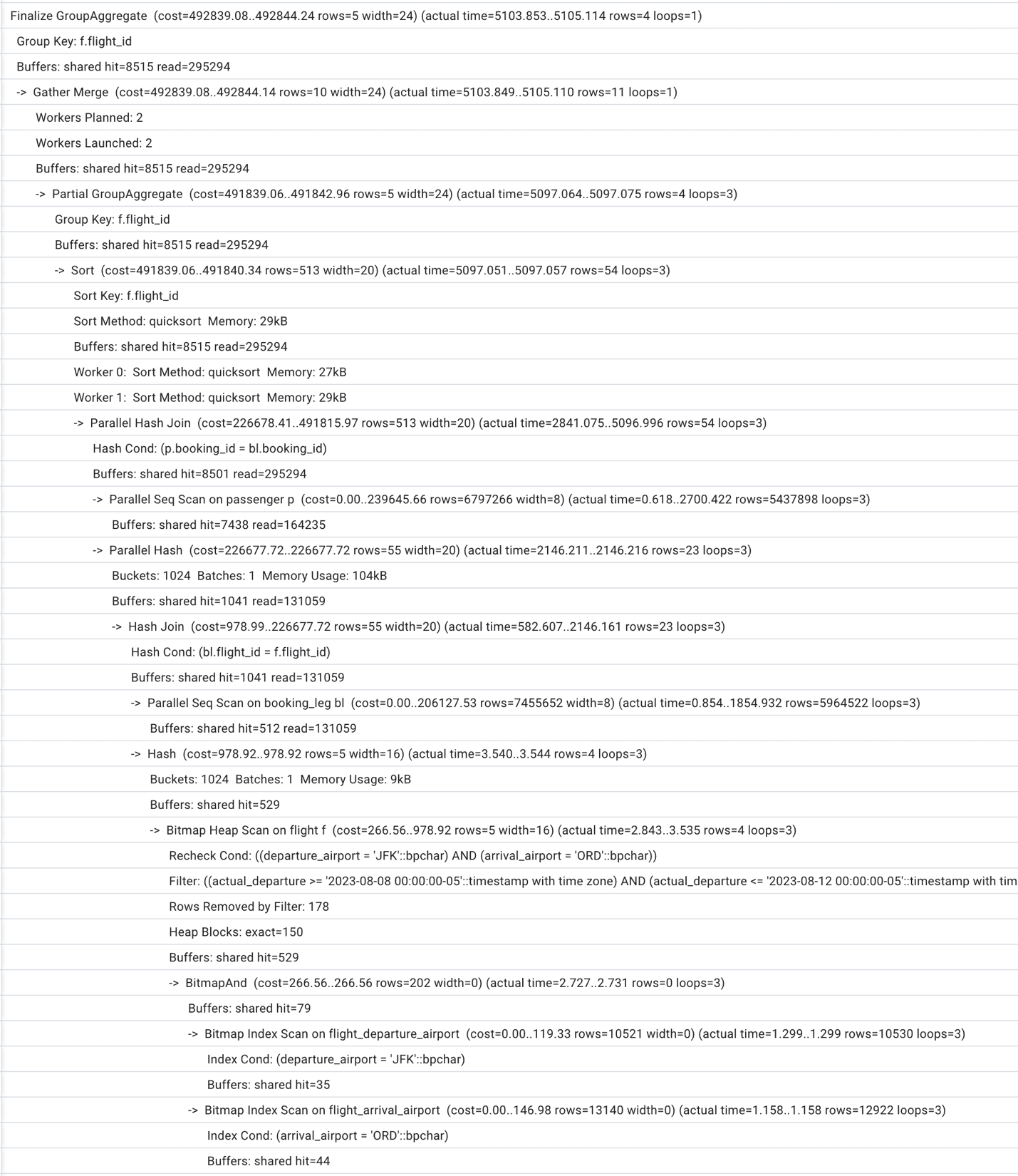
The execution plan for this query is presented in Figure 1. Your results may differ a bit, especially in some of the actual numbers, but should be very similar if you restored a copy of the Air database and added the indexes that were indicated. The query plan will show up in text as a result set in whatever tool you are using.

A screenshot of a computer Description automatically generated with medium confidence

Figure 1. Execution plan with default memory allocations

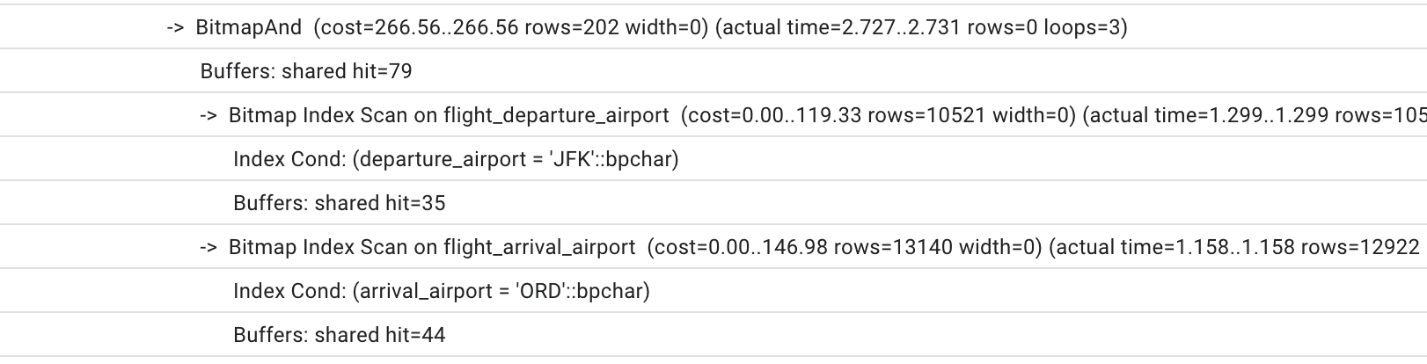
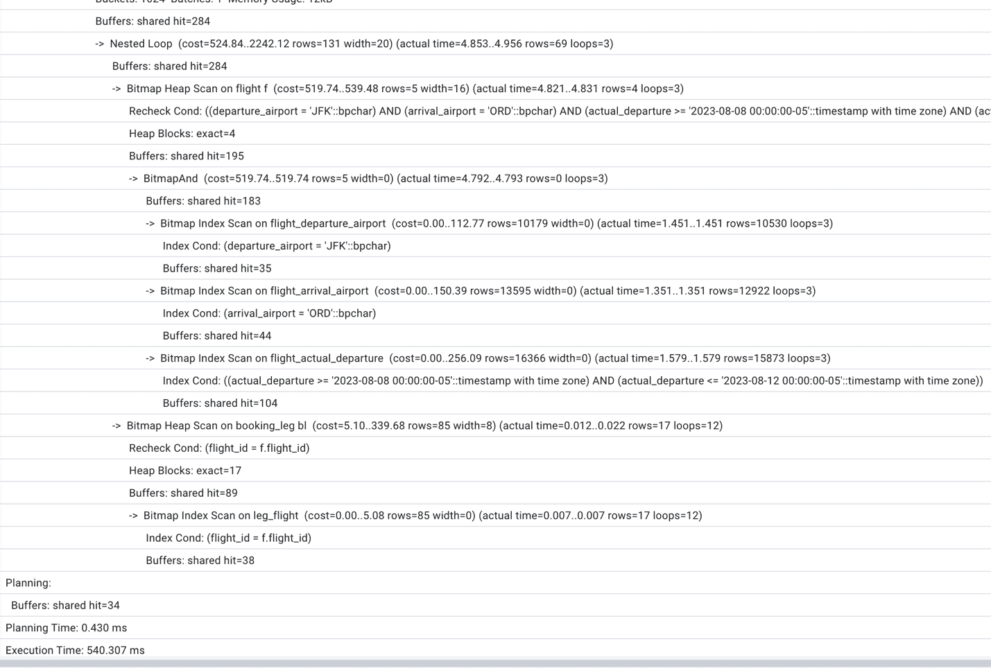
Looking at this query plan, we can see that the optimizer uses two indexes on table flight,

A screenshot of a computer Description automatically generated with low confidence

and then scans all the blocks checking for the actual departure.

A screenshot of a phone Description automatically generated with medium confidence

We can also notice that the number of shared buffers is insufficient (to achieve consistent results, run the same query or EXPLAIN ANALYZE more than once) and that PostgreSQL chooses to run two parallel workers to speed up the process. The total execution time is a little but over one second.

Since we are not modelling the effect of multiple simultaneously running queries, the parameters which might make a material impact on the query execution time are shared_buffers (the change requires restart) and work_mem (can be modified in session). Let’s first try to increase the size of work_mem, then change the shared_buffers parameter to 1 GB, restart the database cluster and repeat the work_mem changes.

Changing the work_mem parameter does not require restart – you can change it locally for a current session and repeat the experiment. Gradually increasing work_mem up to 1GB, we won’t notice any significant changes in the execution plan and execution time. The limiting factor appears to be the insufficient shared_buffers size. We do not see any disk usage which means that there is enough work_mem from the start.

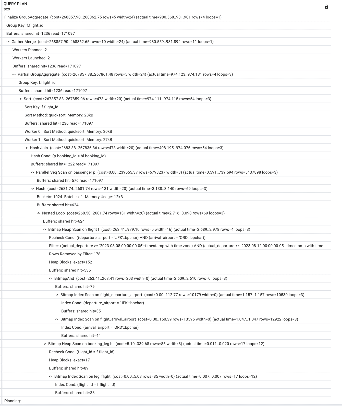
Figure 2 presents the execution plan with 128MB shared_buffers and 500 MB work_mem. Total execution time is fluctuating around 1 sec on my computer for these current parameters. The plan after this change:

A screenshot of a computer Description automatically generated with low confidence

Figure 2. Execution plan with increased work_mem and default shared_buffers

Now, let’s increase shared_buffers to 1GB. TO do this, you will need to edit this parameter in the postgresql.conf file and restart our Postgres instance. Before we start measuring the execution time, we run this query a couple of times making sure that whatever can fit into the shared buffers is there.

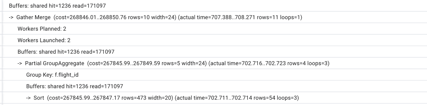
Unfortunately, the execution time decrease will be insignificant. The execution plan will stay the same with the only difference of slightly less reads due to increased shared_buffers (see Figure 3 for a portion of the execution plan)

A screenshot of a computer Description automatically generated with low confidence

Figure 3. A part of the execution plan with increased shared_buffers which shows less reads than on Figure 2.

If we keep increasing the work_mem to 200MB, 500MB, 1 GB, we will notice slow decrease in the execution time, finally getting as low as 750ms. However, we need to be mindful that such increase in work_mem won’t be possible on production server for multiple sessions simultaneously. Anyway, this query does not seem to be too complicated. Are there other ways to improve its performance?

Are there better ways to tune this query?

Looking at all the execution plans which were produced during our experiments, we can notice one major deficiency: Postgres has to read the heap (table rows) in order to find records where the actual departure is within the range from August 8 to August 12. That indicates that an index on this attribute might help. Let’s go ahead and create the missing index:

CREATE INDEX flight_actual_departure
    ON postgres_air.flight (actual_departure);

Immediately, we notice the difference in the execution plan (see Figure 4)

A screenshot of a computer Description automatically generated with medium confidence

Figure 4. Truncated execution plan with index on actual_departure column.

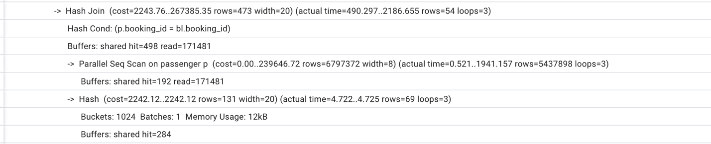
Also, we can see that the execution time finally started to decrease, and we are down to 0.5 sec execution time. However, the difference is still not so dramatic as we would like it to be. Continuing examining the execution plan we notice that Postgres performs a full scan on the passenger table (see Figure 5).

A screenshot of a computer Description automatically generated with low confidence

Figure 5. A part of the execution plan with full table scan.

Looking at the join condition and at the foreign key constraint on the booking_id field, we can conclude that the index on booking_id might help. Indeed, if we create a new index:

CREATE INDEX IF NOT EXISTS passenger_booking_id
    ON postgres_air.passenger (booking_id);

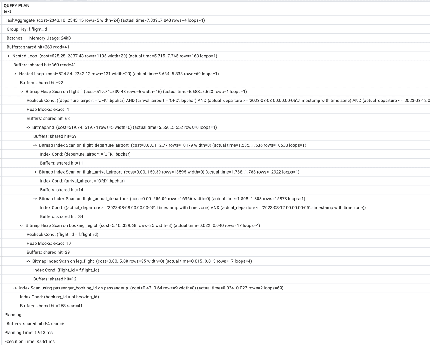
The execution plan will change dramatically – see Figure 6. Now, the total execution time is just 10 ms, which is fifty times shorter than with best possible parameters tuning.

A screenshot of a computer Description automatically generated with medium confidenceFigure 6. Execution plan with two indexes.

More importantly, if we roll back the system parameters to the default settings and reduce the shared_buffers to 128MB, nothing will change either in the execution plan or in the execution time. No wonder – looking closely at the new execution plan in Figure 6, we can see that since we do not need massive table scans, we do not need that many shared buffers!

Other Limitations of Parameters Tuning

When we think about the meaning of the Postgres configuration parameters, it’s important to remember that, in essence, all we are doing is communicating to the query planner what hardware resources it has available. Postgres is agnostic to what is the size of the RAM of the host it is running, what is the type or storage, how many cores are available, and what other systems are running on the same host. We provide some “input parameters” for optimization by setting up parameters to specific values.

For example, if we define shared_buffers=128MB while the host has 16 GB of RAM, the query planner won’t be able to use most of the memory. However, it could choose another way to make queries faster, such as running it with multiple parallel processes, as we saw in Figures 1 – 3.

The opposite is also true. If we have the same 16 GB of RAM, and we allocate 4 GB for shared buffers, and at the same time set default work_mem=200MB and max_connections=700, there are high chance that Postgres will get an “out of memory” error from the operating system.

Another example. The random_page_cost parameter helps the optimizer estimate the cost of index-based access. The default value of 4 in the older Postgres versions reflected the disk characteristics which were available ten years ago. Nowadays, keeping this value at 4 might stop the optimizer from choosing the best execution plan. However, if we reduce this value for the system which utilizes the slow disks, the result will be the opposite.

Conclusion

Although it is important to set up Postgres configuration parameters in the best possible way for a specific system, it is far from enough to achieve the best performance. As we demonstrated, parameters tuning usually helps to improve system performance by ten or twenty percent, and maybe in some cases even more. At the same time, the creation of missing indexes can make the queries run dozen times faster, and the same time reduce resource usage.

In subsequent blog post series, we will talk about multiple techniques that make this optimization possible.


The post When Parameter Tuning is not the Answer appeared first on Simple Talk.


from Simple Talk https://ift.tt/0jmLnI4
via

Monday, July 3, 2023

Beyond Personalization Overcoming Bias in Recommender Systems

Recommender systems are ubiquitous in our everyday lives, providing personalized recommendations on social media, e-commerce platforms, and streaming services. These systems aim to simplify our decision-making by offering products, services, and content tailored to our interests and preferences. However, despite their impressive capabilities, recommender systems are not immune to flaws, and there are concerns about their fairness, particularly in their potential to affect marginalized groups.

This article will delve into the perception of fairness in recommender systems, examining the obstacles to achieving it, and exploring the strategies to mitigate these obstacles.

What is fairness in recommender systems

Under the context of recommender systems, fairness refers to the degree to which the recommendations generated by the system are free from bias and do not favor or discriminate against particular groups of users.

Fairness can be evaluated from different perspectives, including individual fairness, group fairness, and algorithmic fairness.

  • Individual fairness is based on the idea that similar users should receive similar recommendations. This requires that the system does not recommend vastly different items to users with similar preferences, or that it does not recommend the same item to one user while omitting it from another user with similar tastes.
  • Group fairness, requires that the system’s recommendations are distributed fairly among different groups of users, regardless of their demographic characteristics such as age, gender, race, or location1. For instance, a fair recommender system should not exclusively recommend products to one gender over another.
  • Algorithmic fairness concerns the fairness of the underlying algorithms and data used to make recommendations. This ensures that the recommendations generated by the system do not perpetuate existing biases or discrimination. For example, if a movie recommendation system disproportionately recommends films by male directors, then the system may be perpetuating a gender bias2.

Evaluating and achieving fairness in recommender systems is a complex and ongoing challenge, as there is no one-size-fits-all approach to ensuring fairness. However, by understanding and addressing the different perspectives of fairness, we can design and implement recommender systems that are more equitable and unbiased for all users.

Challenges in achieving fairness in recommender systems

In this section, I will cover some of the primary fairness issues that come up when building a recommender system.

Data Bias

Achieving fairness in recommender systems is a challenging task, as there are numerous obstacles that need to be overcome. One of the most significant obstacles is data biases3, which can result in unfair and discriminatory recommendations. Recommender systems are trained on historical user data, which may contain biases and stereotypes. These biases can be reflected in the recommendations generated by the system, perpetuating existing inequalities.

For example, if a movie recommendation system only recommends films by a specific race or ethnicity, it may reinforce existing biases and limit diversity in film choices. To address this challenge, data preprocessing techniques can be used to remove or mitigate the effects of biases. Oversampling underrepresented groups, reweighting the data, or using techniques such as adversarial debiasing can help balance the data and reduce the impact of biases.

Lack of Diversity

Another obstacle for achieving fairness in recommender systems is the lack of diversity in recommendations. Recommender systems can suffer from a lack of diversity, as they may recommend similar items to users with similar tastes, which can create filter bubbles and limit users’ exposure to new and diverse content. This can have implications for underrepresented groups, as their interests and preferences may not be reflected in the recommendations they receive.

To address this challenge, various techniques can be used to promote diversity, such as incorporating diversity metrics into the recommendation process or providing users with serendipitous recommendations that introduce them to new content. For example, a music recommendation system can use diversity metrics to recommend music that is less popular but aligns with a user’s tastes.

Cold Start Problem

Recommender systems may struggle to provide personalized recommendations to new users who have little to no historical data. This can put these users at a disadvantage compared to users with established profiles and more data for the system to work with. This is known as the cold start problem.

One way to address this challenge is to use content-based recommendations that leverage the features of items to make recommendations, rather than relying solely on historical user data. For example, a music recommendation system can use audio features like tempo, key, and genre to recommend songs to users who have not yet established their preferences.

Privacy Concerns

Recommender systems require access to users’ personal data, such as their browsing history, purchase history, or location, to make recommendations. This can raise privacy concerns and undermine user trust in the system. To address this challenge, privacy-preserving techniques such as differential privacy can be used to protect users’ data while still providing accurate recommendations. For example, a recommendation system can use differential privacy to add random noise to the data before processing it, making it difficult for a potential attacker to identify specific users’ data while still maintaining the accuracy of the recommendations. Additionally, recommender systems can be transparent about their data collection practices and offer users the ability to opt out of data collection or delete their data at any time.

Approaches to achieving fairness in recommender systems

Despite these challenges, there are several approaches to achieve fairness in recommender systems. Some of these approaches will be covered in the following section.

Algorithmic modifications

One approach to achieving fairness in recommender systems is to modify the algorithms used by the system to ensure fairness. For example, one could modify the objective function to explicitly include fairness constraints or incorporate diversity metrics into the recommendation process.

import numpy as np
from sklearn.metrics.pairwise import cosine_similarity
def fair_collaborative_filtering(user_item_matrix, 
                                    fairness_constraint):
    """
    Compute fair collaborative filtering recommendations.
    
    Args:
        user_item_matrix (np.array): The user-item matrix.
        fairness_constraint (float): The fairness constraint, 
                                           between 0 and 1.
        
    Returns:
        np.array: The fair collaborative 
                  filtering recommendations.
    """
    user_similarity = cosine_similarity(user_item_matrix)
    item_similarity = cosine_similarity(user_item_matrix.T)
    
    # Compute the fairness-corrected item similarity matrix
    fair_item_similarity = (1 - fairness_constraint) * 
                     item_similarity + fairness_constraint *        
                         np.identity(item_similarity.shape[0])
    
    # Compute recommendations using the fair item 
    #                            similarity matrix
    recommendations = user_item_matrix.dot(fair_item_similarity)
    
    return recommendations

This function first calculates user and item similarity matrices using cosine similarity. Then, it computes the fairness-corrected item similarity matrix by blending the original item similarity matrix with an identity matrix, guided by the fairness constraint parameter. Finally, it calculates recommendations using the fair item similarity matrix.

User feedback

User feedback is a crucial aspect of building fair recommender systems. User feedback can help the system learn from its mistakes and improve its recommendations over time. Explicit feedback, where users rate or provide feedback on the recommendations they receive, can be particularly helpful in identifying and addressing biases in the system.

To incorporate user feedback into the recommendation process, several techniques can be used, such as:

  1. Collaborative filtering: This involves using user feedback to compute similarity scores between users and items. The similarity scores can then be used to generate recommendations for new users. Using the movie recommender system as an example, we have a user-item matrix containing the user’s rating to a given movie. In the example below, User_A gives Movie_1 a rating of 4. For any new user, we can find a similar user in the existing user-item matrix, and bootstrap a rating the new user might give to a movie.

User-Item Matrix


Movie_1

Movie_2

Movie_3

Movie_4

User_A

4


5


User_B


2


1

User_C


5


New User

3 ?

?

?

To operationalize this in python:

import pandas as pd
from sklearn.metrics.pairwise import cosine_similarity

# load user feedback
feedback = pd.read_csv('feedback.csv')

# compute similarity scores between users and items
user_matrix = feedback.pivot_table(index='user_id', columns='item_id', 
                               values='rating', fill_value=0)
user_similarity = cosine_similarity(user_matrix)

# generate recommendations for a new user
new_user_id = 123
new_user_ratings = [4, 0, 0, 2, 0, 0, 5, 0, 3, 0]
new_user_similarities = user_similarity[new_user_id]
recommendations = user_matrix.dot(new_user_similarities).div
                                  (user_similarity.sum(axis=1))
recommendations = recommendations.sort_values(ascending=False)
  1. Active learning: This involves using user feedback to iteratively refine the recommendation model. The system starts with a simple model and asks users for feedback on the recommendations. The feedback is used to improve the model, and the process is repeated until the model reaches a satisfactory level of accuracy. For example, a music recommendation system can use active learning to improve the accuracy of its recommendations by asking users for feedback on the recommended songs.
import pandas as pd
from sklearn.linear_model import LogisticRegression
from sklearn.metrics import accuracy_score

# load user feedback
feedback = pd.read_csv('feedback.csv')

# split feedback into training and testing sets
train = feedback.sample(frac=0.8, random_state=123)
test = feedback.drop(train.index)

# initialize model
model = LogisticRegression()

# train model on initial training set
model.fit(train[['user_id', 'item_id']], train['rating'])

# evaluate model on testing set
predictions = model.predict(test[['user_id', 'item_id']])
accuracy = accuracy_score(test['rating'], predictions)

# ask users for feedback on the recommendations
new_feedback = get_user_feedback()

# incorporate feedback into the model
model.fit(new_feedback[['user_id', 'item_id']], new_feedback['rating'])

Transparency

Transparency and accountability are critical for promoting fairness in recommender systems. By providing users with more information about how the system works, including the algorithms used and the data sources, and allowing users to opt out of certain types of recommendations, we can ensure that users are more informed about the recommendations they receive and have more control over their experience.

To promote transparency and accountability in recommender systems, several techniques can be used, such as:

  1. Explainability: This involves providing users with explanations for the recommendations they receive. For example, a movie recommendation system can provide users with information on how the recommended movies are related to the user’s viewing history or preferences.
import pandas as pd
from sklearn.ensemble import RandomForestRegressor
import shap

# load data
data = pd.read_csv('data.csv')

# train model
model = RandomForestRegressor()
model.fit(data[['user_age', 'item_rating']], data['rating'])

# generate explanations for a prediction
user_age = 30
item_rating = 4.5
prediction = model.predict([[user_age, item_rating]])
explainer = shap.TreeExplainer(model)
shap_values = explainer.shap_values([[user_age, item_rating]])
shap.initjs()
shap.force_plot(explainer.expected_value, shap_values[0], 
  [[user_age, item_rating]], feature_names=['user_age', 
                                            'item_rating'])
  1. Opt-out options: This involves providing users with the ability to opt out of certain types of recommendations. For example, a music recommendation system can provide users with the ability to opt out of recommendations based on their listening history.
import pandas as pd
from sklearn.metrics.pairwise import cosine_similarity

# load user data
user_data = pd.read_csv('user_data.csv')

# load item data
item_data = pd.read_csv('item_data.csv')

# compute similarity matrix between users and items
user_matrix = user_data.drop(columns=['user_id']).values
item_matrix = item_data.drop(columns=['item_id']).values
user_item_similarity = cosine_similarity(user_matrix, item_matrix)

# compute personalized recommendations for a user
user_id = 123
recommendations = user_item_similarity[user_id].argsort()[::-1][:10]

# provide user with opt-out options
opt_out_items = [456, 789]
recommendations = 
   [r for r in recommendations if r not in opt_out_items][:5]

Hybrid Recommendations

This involves combining different recommendation techniques such as content-based, collaborative filtering, or knowledge-based recommendations to provide more accurate and diverse recommendations. The system can use user feedback to adapt the weightings of each technique to improve the accuracy of recommendations for individual users. For example, an e-commerce recommendation system can use a hybrid approach to recommend products based on a combination of user preferences and the popularity of the products.

import pandas as pd
from sklearn.metrics.pairwise import cosine_similarity

# load user feedback
feedback = pd.read_csv('feedback.csv')

# initialize models
model_content = ContentBasedModel()
model_cf = CollaborativeFilteringModel()
model_kb = KnowledgeBasedModel()

# train models on feedback
model_content.fit(feedback)
model_cf.fit(feedback)
model_kb.fit(feedback)

# combine predictions from multiple models
user_id = 123
item_id = 456
weight_content = 0.4
weight_cf = 0.4
weight_kb = 0.2
prediction_content = model_content.predict(user_id, item_id)
prediction_cf = model_cf.predict(user_id, item_id)
prediction_kb = model_kb.predict(user_id, item_id)
prediction = (prediction_content * weight_content) +
    (prediction_cf * weight_cf) + (prediction_kb * weight_kb)

# ask user for feedback on the recommendation
rating = get_user_feedback()

# update weights based on user feedback
if rating > 3:
    weight_content += 0.1
    weight_cf += 0.1
    weight_kb -= 0.1
elif rating < 3:
    weight_content -= 0.1
    weight_cf += 0.1
    weight_kb += 0.1

# recompute prediction with updated weights
prediction = (prediction_content * weight_content) + 
     (prediction_cf * weight_cf) + (prediction_kb * weight_kb)

Conclusion

Recommender systems have the potential to provide personalized and relevant recommendations to users, but they also raise concerns about fairness and discrimination. Achieving fairness in recommender systems is a complex and ongoing challenge that requires a multi-disciplinary approach, such as computer science, data science, ethics, and social science. By combining their expertise and perspectives, it becomes possible to develop more equitable algorithms, systematically identify and address biases, and create a fairer digital environment for users and content creators alike.

  1. Michael D. Ekstrand, Mucun Tian, Ion Madrazo Azpiazu, Jennifer D. Ekstrand, Oghenemaro Anuyah, David McNeill, and Maria Soledad Pera, “All The Cool Kids, How Do They Fit In?: Popularity and Demographic Biases in Recommender Evaluation and Effectiveness,” in Proceedings of the Conference on Fairness, Accountability, and Transparency (FAT* ’18), 2018, pp. 172-186.
  2. F. Maxwell Harper and Joseph A. Konstan, “The MovieLens Datasets: History and Context,” ACM Transactions on Interactive Intelligent Systems (TiiS) 5, no. 4 (2015): 19:1-19:19.
  3. Alexandra Olteanu, Carlos Castillo, Fernando Diaz, and Emre Kıcıman, “Social Data: Biases, Methodological Pitfalls, and Ethical Boundaries,” Frontiers in Big Data 2 (2019): 13.


The post Beyond Personalization, Overcoming Bias in Recommender Systems appeared first on Simple Talk.


from Simple Talk https://ift.tt/nr6HPaA
via