SQL Server Row Level Security Deep Dive. Part 6 – RLS Attack Mitigations

As seen in the previous section, there are several ways bad actors can attempt to bypass RLS. Attacks range from removing RLS, getting data from other systems or straight brute-force methods using side-channel attacks. Mechanisms exist for each potential attack that allow you to avoid the attack or monitor for the attack when avoidance isn’t possible. This section covers those mitigations.

RLS can be bypassed or attacked using several broad categories. These include direct attacks, where RLS is modified in a malicious fashion or disabled, indirect attacks where information can be gathered without modifying the underlying RLS, and side-channel attacks that use specially crafted queries to derive data from RLS protected tables. Refer to the previous section of this series, RLS Attacks, for a full explanation of each attack type.

Excessive errors

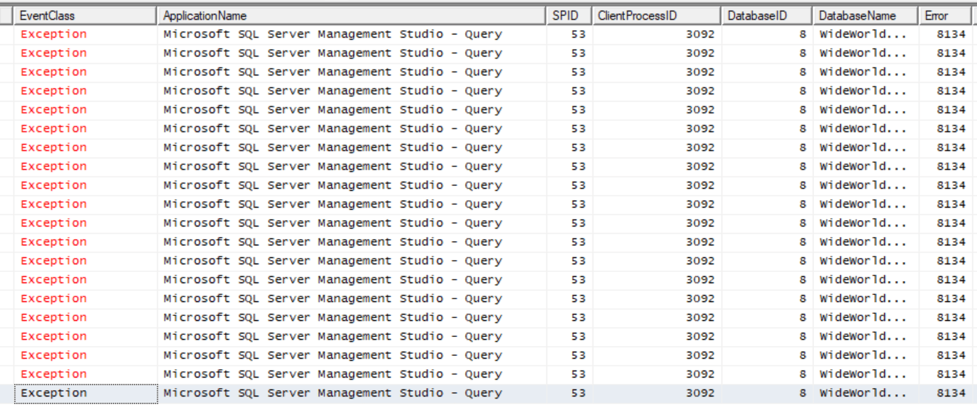
Side channel attacks, with the current vulnerability, rely on forcing runtime errors. The exact error is 8134, divide by zero. This is an error that can be captured, allowing administrators to monitor for possible attacks. There are several ways to capture these errors and the method you employ will depend on your environment, standards, and preferences. When taking advantage of the divide by zero attack, thousands or even hundreds of thousands of errors are generated, leaving a large attack footprint. This makes it easier to see the attack – it really sticks out in the logs if you are checking for it.

SQL Trace

The error raised by divide-by-zero attacks is 8134. If a trace is created, the preferred method is using sp_trace_create. Using SQL Profiler is a good way to prototype a trace, but there are some disadvantages. Profiler sends all data over the network, increasing the performance cost. It also runs on a client machine, which must be on and connected all the time (or Profiler must be running on the server, which takes additional server resources) and can’t be configured to run automatically. Profiler is just a front-end for trace, so it’s a good idea to learn how to create a simple trace.

The following shows how this can be configured in profiler.

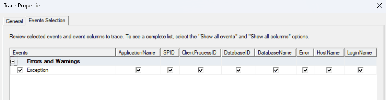
This example uses TSQL to create a trace capturing exceptions. As noted above, profiler also creates a trace, but it is more resource heavy.

DECLARE                @ReturnCode                     int
                        ,@TraceID                       int
                        ,@maxfilesize           bigint          = 128
                        ,@traceoptions          int                     = 2
                        ,@stoptime                      datetime
                        ,@FileName                      nvarchar(256)
SELECT @FileName = 'C:\Temp\RLSExceptions_' + replace(replace(replace(replace(convert(varchar(50),getdate(),100),'-',''),' ','_'),':',''),'__','_')
-- Create the trace with the name of the output file - .trc extension is added to filename
EXEC @ReturnCode = sp_trace_create @TraceID OUTPUT, 2, @FileName, @maxfilesize, NULL 
if (@ReturnCode <> 0) GOTO error
-- Set the events
declare @on bit
set @on = 1
-- 33   Exception       Indicates that an exception has occurred in SQL Server
EXEC sp_trace_setevent @TraceID, 33, 3, @on             --DatabaseID
EXEC sp_trace_setevent @TraceID, 33, 6, @on             --NTUserName
EXEC sp_trace_setevent @TraceID, 33, 8, @on             --HostName
EXEC sp_trace_setevent @TraceID, 33, 9, @on             --ClientProcessID
EXEC sp_trace_setevent @TraceID, 33, 10, @on    --ApplicationName
EXEC sp_trace_setevent @TraceID, 33, 11, @on    --LoginName
EXEC sp_trace_setevent @TraceID, 33, 12, @on    --SPID
EXEC sp_trace_setevent @TraceID, 33, 13, @on    --Duration
EXEC sp_trace_setevent @TraceID, 33, 14, @on    --StartTime
EXEC sp_trace_setevent @TraceID, 33, 15, @on    --EndTime
EXEC sp_trace_setevent @TraceID, 33, 27, @on    --Event Class
EXEC sp_trace_setevent @TraceID, 33, 31, @on    --Error
-- Ordinarily filters would be set here.
-- Capturing only the exception doesn't require any filters
-- unless known errors are regularly encountered
-- Set the trace status to start
EXEC sp_trace_setstatus @TraceID, 1
-- display trace id for future references
SELECT
        TraceID                 = @TraceID
        ,TraceName              = @FileName + '.trc'
GOTO FINISH
ERROR:
SELECT ErrorCode=@ReturnCode
FINISH: 
PRINT 'TRACE ' + convert(varchar(5),@TraceID) + ' created successfully'
PRINT 'TRACE name: ' + @FileName + '.trc'
GO

Output using a query to pull the results is shown below.

DECLARE 
        @curr_tracefilename                     VARCHAR(500)
        ,@base_tracefilename            VARCHAR(500)
        ,@indx                                          INT
--Note that the trace ID may vary if other traces are running
--Use the ID output during trace creation
SELECT @base_tracefilename = path
FROM sys.traces ST
WHERE ST.id = 2
SELECT
        ClientProcessID
        ,ApplicationName
        ,SPID
        ,StartTime
        ,EventClass
        ,Error
FROM::fn_trace_gettable(@base_tracefilename, DEFAULT) GT

Sample output from the trace when a brute force attack is running

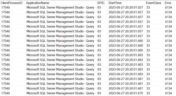
SQL Trace Deprecation

Microsoft documentation warns that trace functionality will be removed in a future version of SQL Server. Take this into consideration when selecting your method for monitoring potential RLS attacks.

Extended events

In Azure databases, as well as all other SQL instances, extended events can be used to capture error 8134. I find extended events harder to work with and slower to query, but once configured they work well. They also only run on the server which helps performance. When they are setup in the GUI, they can be configured to show live results, but this wouldn’t be the method for active attack monitoring. The following shows how to setup an extended event to capture errors .

DROP EVENT SESSION RLSErrors ON SERVER
GO
--Extended even targeting errors
CREATE EVENT SESSION RLSErrors ON SERVER
ADD EVENT sqlserver.error_reported(
        ACTION(
                sqlserver.client_hostname
                ,sqlserver.database_id
                ,sqlserver.database_name
                ,sqlserver.nt_username
                ,sqlserver.sql_text
                ,sqlserver.tsql_stack
                ,sqlserver.username
)
) --Location to store data. Several options are available, check documentation for the best fit
ADD TARGET package0.event_file(SET filename=N'C:\Temp\RLSErrors.xel')
WITH (
        MAX_MEMORY=4096 KB
        ,EVENT_RETENTION_MODE=ALLOW_SINGLE_EVENT_LOSS
        ,MAX_DISPATCH_LATENCY=1 SECONDS
        ,MAX_EVENT_SIZE=0 KB
        ,MEMORY_PARTITION_MODE=NONE
        ,TRACK_CAUSALITY=OFF
        ,STARTUP_STATE=OFF
)
GO
 
ALTER EVENT SESSION RLSErrors ON SERVER
STATE = START;
GO

For the above extended event, this will pull the errors. I didn’t limit the query to error 8134 alone, but it would be reasonable to do so.

;
WITH XE_CTE AS (
        SELECT
                CONVERT(XML,event_data) EventData
        FROM sys.fn_xe_file_target_read_file('C:\Temp\RLSErrors*.xel',NULL,NULL,NULL)
)
,DECODED_CTE AS (
        SELECT
                EventData.value('(/event/data[@name=''error_number'']/value)[1]','varchar(max)')                                ErrorNumber
        FROM XE_CTE
)
SELECT 
        ErrorNumber
        ,COUNT(*)                       ErrorCount
FROM DECODED_CTE
WHERE ErrorNumber               = 8134
GROUP BY ErrorNumber

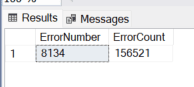
Results from the above query. This was generated by testing the brute-force side-channel attack script with 100 rows. As seen below, over 156 thousand errors are produced for this relatively small dataset. If you see numbers like this, you should dig deeper into what is happening in your system and rule out an RLS attack.

Server or Database Audits

SQL Server instances can use server and database audits to log queries against the server and databases on that server. Auditing for Azure SQL can be used to do the same thing against Azure databases and Azure Synapse. This can be useful for forensic analysis after an attack or even to determine that an attack has occurred. It can capture all queries against a database and it can also capture DBCC commands against a database if that vulnerability is a concern.

A benefit of using audits is that they aren’t limited to monitoring for RLS attacks. They can be used for a wide range of monitoring functions. Reports can be created for audit records making it a simple process to search for issues. If you are already using audits this is a good method to check for RLS related attacks.

SQL Advanced Threat Protection

SQL Advanced Threat Protection is an automated, relatively hands-off method to watch for attacks against SQL Server in Azure. The documentation lists SQL injections specifically, and general suspicious activity and vulnerabilities as target threats. It may catch RLS attacks in the future or certain RLS attacks, but in my testing, I didn’t get any warnings via this tool. It looks like a very useful method for capturing potential security issues, but you will want to supplement this with your own audits for now if RLS is part of your environment.

Performance Changes

Brute force attacks are not considerate of performance. This can potentially be used to detect an attack in action. The primary method to check is CPU usage. In lower-level Azure tiers, DTU usage can also be monitored.

Excessive CPU Usage

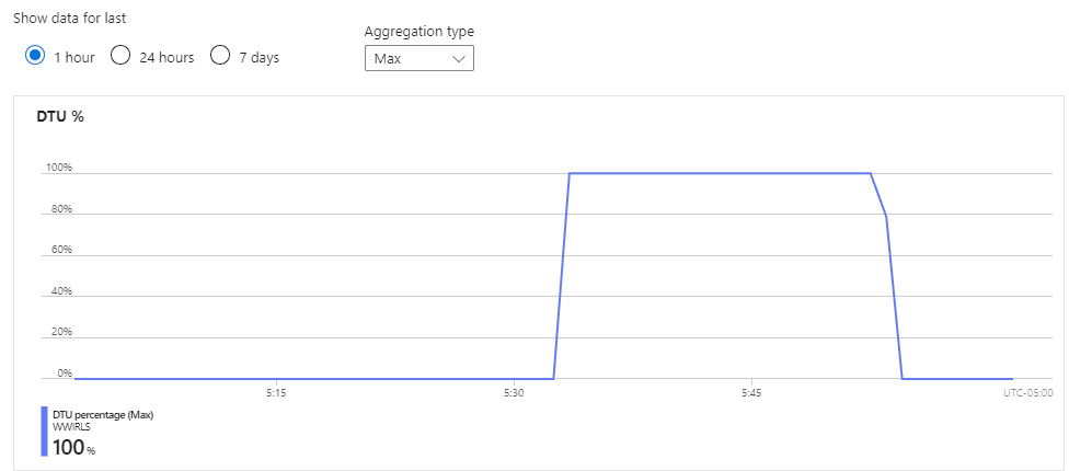
Brute force attacks cause CPU usage to spike. Depending on your configuration, it may be noticeable or it may blend into the background. In my test Azure SQL database environment, with the minimum DTUs, it was very noticeable. The DTU overview showed 100% utilization during an unregulated side-channel attack.

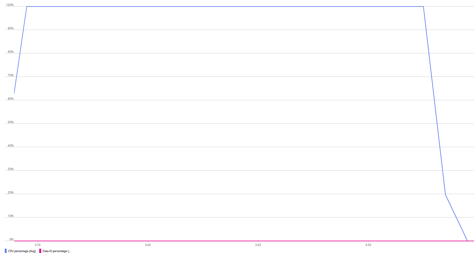
The CPU metric on the monitoring page also showed 100% utilization for this low tier SQL database.

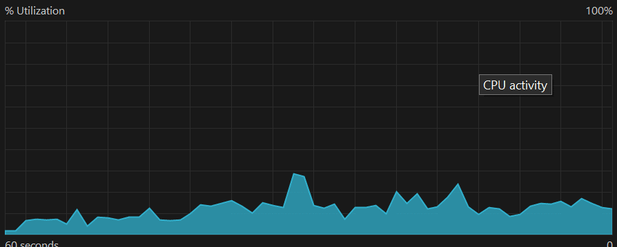
My local workstation with SQL Server 2022 Developer Edition showed an increase in CPU usage, but not something I would probably notice or be concerned about. If RLS attacks are a concern on your system, you will want to see how your configuration performs when under attack.

This is still not a foolproof method for detecting these attacks. If an attacker is patient, they would just put a WAITFOR command in their attack to limit the impact of their script. It will still throw the 8134 (divide by zero) error, but the errors would be spread out over time. This is very similar to network port scans. An attacker will wait between scanning each port or even change IP addresses during the scan. Firewalls have evolved to detect these attacks. Your methods will need to evolve too and you will need to be aware of this method when protecting your systems.

--Sleep for 1 second
--Will reduce CPU usage and space out errors
--at the expense of attack speed
WAITFOR DELAY '00:00:01'

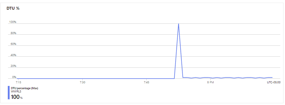
This limits the CPU impact of the attack almost entirely, but in the low performance tier, it still spikes the CPU to 100% during the initial processing of the primary key. After that processing, the impact is negligible, but the process is limited to 1 character discovered every second (or whatever interval is selected). Given that there were 156,521 errors generated, it would take almost 2 full days to reveal the protected data in the first 100 rows. Making the delay 50 milliseconds provided the data in a more reasonable time and the CPU was still below 20%. The following graph shows the impact of a 1 second delay.

Attack monitoring

The above tactics can be used to capture attacks. To alert administrators, a few methods can be used. Each method should look for excessive numbers of error 8134. Depending on your system and needs, you may also look for excessive CPU usage, specific DBCC commands, disabling RLS, or even data changes to RLS configuration tables. You will need to incorporate the scripts appropriate for your environment and perceived threat surface and create alerts for each of these.

SQL Agent Job

If a SQL Trace is used, SQL Agent is a potential method to monitor for attacks. If the error count exceeds a defined threshold during a time period, administrators can be notified. It can also be used against extended events, provided the server is on premises or a managed instance.

Agent jobs can also run queries looking for changes to your RLS tables or anything else that can be queried. RLS tables are a good use case for temporal tables. If the RLS configuration is a temporal table, a simple query will show any changes during a given time period. As mentioned previously, RLS is not prescriptive, so you will need to create scripts based on your implementation.

Elastic Job

In a pure Azure environment, Elastic Jobs can be used in a similar manner to SQL Agent jobs. This could be used to query extended events or RLS changes. Since SQL Trace is not available in Azure database, you wouldn’t likely use it for that.

Elastic Job Warning

At the time of this writing, Elastic Jobs are still in development. They have been available for quite a while and appear to be part of the ongoing Azure offerings, but there is no guarantee they will be implemented officially.

External Scheduler / Custom Code

Any external scheduler or custom code that can run SQL queries and send email or other notifications to administrators can be used to monitor for attacks. This will be specific to your environment and the exact method doesn’t matter. My general recommendation is to follow your existing patterns, taking into account future needs. Don’t build a custom solution if you have an existing scheduler or if you have SQL Agent available.

Code repo with history

All modern code repositories maintain history and can be used to show when changes happened and who made the changes. This won’t stop attacks by itself, but it will help with a post-attack analysis. It is also a deterrent to direct code attacks via an automated pipeline. If security is misconfigured, a developer / attacker could remove history in the repo. This is another case in the enterprise for minimum viable security.

Code reviews

Code reviews are a standard practice and a good method to find errors in access predicates, both intentional and unintentional. Microsoft documentation mentions taking care with users configured as policy managers. They can change and bypass RLS configurations. The same is true for developers, especially for automated or non-monitored deployments. Carefully review access predicates and security policy changes. Malicious changes are a risk, but a more likely scenario is code misconfigurations. Either case results in the potential for unauthorized access.

Audit for changes to security objects

Existing access predicates and security policies should be regularly audited and validated. This is to ensure they are still enabled and that the code hasn’t changed. The more sensitive the system and data, the more frequently it should be confirmed. It is useful, and I would say required, to know the expected configuration. Audits can be managed in several ways and some options are detailed below.

Tables with RLS applied can be verified using SQL metadata queries. Tables with RLS and tables without RLS applied, predicate definitions, and columns used for RLS can all be checked very easily. The same types of queries can also examine security policies and access predicates.

Depending on your code repository, you can also compare the committed code to your deployed database objects. There should be a very limited set of accounts that can change objects in a production environment, but it can be worth auditing. This would also check for changes in addition to RLS objects making it even more useful.

SQL metadata can also be used to look for changes to RLS related objects. This is easier if you use standard naming conventions and a separate schema. The modify_date will show when RLS objects have changed. It will also show if an object is dropped and recreated with the same name. There are also trace and extended events that can check for changes to objects. The following example query shows all objects in the RLS schema changed within the last day.

SELECT
        SS.name                 SchemaName
        ,SO.name                ObjectName
        ,SO.create_date
        ,SO.modify_date
        ,DATEADD(dd,-10,SO.modify_date)
        ,DATEDIFF(dd,SO.modify_date,GETDATE())
FROM sys.schemas SS
        INNER JOIN sys.objects SO
                ON SS.schema_id         = SO.schema_id
WHERE SS.name                           = 'RLS'
        AND SO.type                             IN ('IF','SP')          --IF = SQL Inline Table Valued Function, SP = Security Policy
        AND DATEDIFF(dd,SO.modify_date,GETDATE()) <= 1               --RLS objects changed in the last day. Change to a time interval and value appropriate for your environment
ORDER BY SO.modify_date DESC

Azure Alerts

Azure alerts can be used to check for performance issues and alert administrators. It usually won’t be an indication of an ongoing attack, but that is one possible reason for major changes in CPU or disk performance. During my testing I saw changes to CPU. This would be an area of interest for any administrator, even if an attack isn’t suspected.

RLS Support and Administration Scripts

 RLS is easy to validate using metadata scripts. The following samples show a few ways to check your RLS configuration.

Objects with RLS applied

The following shows all security policies and access predicate details. This is useful for reviewing security at a database level.

SET NOCOUNT ON
;
WITH ACCESS_PREDICATES AS (
        SELECT
                SP.object_id
                ,SP.target_object_id
                ,SS.value                               AccessPredicateName
        FROM sys.security_predicates SP
                CROSS APPLY string_split(SP.predicate_definition,N'(') SS
        WHERE SS.value <> ''
                AND SS.value NOT LIKE '%))'
)
SELECT
        SS.name                                                         SchemaName
        ,SO.name                                                        TableName
        ,SSSP.name                                                      SecurityPolicySchema
        ,SSP.name                                                       SecurityPolicyName
        ,SSP.type_desc                                          SecurityPolicyDescription
        ,SSP.is_enabled                                         SecurityPolicyIsEnabled
        ,AP.AccessPredicateName
        ,SP.predicate_definition                        AccessPredicateDefinition
        ,SP.operation_desc
        ,SP.predicate_type_desc
FROM sys.schemas SS
        INNER JOIN sys.objects SO
                ON SS.schema_id                 = SO.schema_id
        INNER JOIN sys.security_predicates SP
                ON SO.object_id                 = SP.target_object_id
        INNER JOIN sys.security_policies SSP
                ON SP.object_id                 = SSP.object_id
        INNER JOIN sys.schemas SSSP
                ON SSP.schema_id                = SSSP.schema_id
        LEFT JOIN ACCESS_PREDICATES AP
                ON SP.object_id                 = AP.object_id
                AND SP.target_object_id = AP.target_object_id
ORDER BY
        SS.name
        ,SO.name
        ,SSP.name
GO

Tables without RLS

The following can be used to show all tables in a database without a security predicate assigned. This is useful for finding new tables that were not properly assigned RLS and also for finding tables where RLS has been removed.

SET NOCOUNT ON
DECLARE @Exclusions TABLE (
        SchemaName                                                      varchar(255)
)
--Optionally - exclude the following schemas from the search
--The RLS schema would not have a security predicate assigned
--rather, regular users would not be able to access it at all.
INSERT INTO @Exclusions (
        SchemaName
)
VALUES 
        ('etl')
        ,('RLS')
        ,('ssrs')
SELECT
        SS.name                                                         SchemaName
        ,SO.name                                                        TableName
FROM sys.schemas SS
        INNER JOIN sys.objects SO
                ON SS.schema_id                 = SO.schema_id
        LEFT JOIN sys.security_predicates SP
                ON SO.object_id                 = SP.target_object_id
        LEFT JOIN @Exclusions EX
                ON SS.name                              = EX.SchemaName
WHERE SO.type                                   = 'u'
        AND EX.SchemaName                       IS NULL
        AND SP.object_id                        IS NULL
ORDER BY
        SS.name
        ,SO.name
GO

Specific column without RLS

Sometimes you only want to look for a specific column without RLS applied. In larger systems, this can save time and also allows team members without a full understanding of RLS to help run pointed audits. It is useful to perform these checks in production environments with many team members or rapidly shifting teams. It is easy for tables to be inserted into production without RLS in these scenarios. This script is a modification of the previous with additional parameters added to limit the columns searched.

SET NOCOUNT ON
DECLARE @Exclusions TABLE (
        SchemaName                                                      varchar(255)
)
--Limit the columns
--ExactMatch = 1 matches the full name
--ExactMatch = 0 performs a wildcard search
DECLARE @RLSColumn              varchar(255)    = 'SupplierID'
        ,@ExactMatch            bit                             = 1
--Optionally - exclude the following schemas from the search
--The RLS schema would not have a security predicate assigned
--rather, regular users would not be able to access it at all.
INSERT INTO @Exclusions (
        SchemaName
)
VALUES 
        ('etl')
        ,('RLS')
        ,('ssrs')
SELECT
        SS.name                                         SchemaName
        ,SO.name                                        TableName
        ,SC.name                                        ColumnName
FROM sys.schemas SS
        INNER JOIN sys.objects SO
                ON SS.schema_id                 = SO.schema_id
        INNER JOIN sys.columns SC
                ON SO.object_id                 = SC.object_id
        LEFT JOIN sys.security_predicates SP
                ON SO.object_id                 = SP.target_object_id
        LEFT JOIN @Exclusions EX
                ON SS.name                              = EX.SchemaName
WHERE SO.type                                   = 'u'
        AND EX.SchemaName                       IS NULL
        AND SP.object_id                        IS NULL
        AND SC.name                                     LIKE CASE WHEN @ExactMatch = 1 THEN @RLSColumn ELSE '%' +  @RLSColumn + '%' END
ORDER BY
        SS.name
        ,SO.name
GO

Summary and analysis

RLS is a great way to add a layer of protection to a SQL Server database. It is not the most secure option but it is relatively easy to implement, provides a method to greatly simplify reporting and query needs, and may be secure enough, depending on requirements. The ease of implementation makes is very enticing for internal reporting solutions. It can greatly decrease the number and complexity of reports required.

Layer of security

RLS is an additional layer of security that can be added to a solution. It is not a replacement for other authorization methods, but an enhancement that can be very useful in reporting and warehousing scenarios. Configured correctly, it can also work in transactional applications when used with SESSION_CONTEXT as a means of limiting data seen by particular users.

Hire trusted admins

System administrators and developers must be trusted to some degree. It is still possible, and sometimes required, to audit their activities, but the relationship with administrators must begin with trust. If users with elevated privileges are not trusted, they should not be in the system. Period. But that trust must be earned over time and reinforced with good decisions and successful projects. Administrators and developers have access to logon scripts, backups, monitoring, object code, change requests, and many other methods to directly impact databases and secure data. It is very difficult to prevent bad actors in these categories from gaining extra or unauthorized access. That is where audits can help fill the gap for security requirements.

Consider alternatives if the use case fits

There are several alternatives to RLS. These alternatives were the only way to segregate data by user before RLS was added to SQL Server. Some project use cases fit better with these custom solutions than with RLS. Alternatives include separate views or stored procedures for different users, separate reports, or other custom code.

Locking the data down excessively can potentially encourage data exports, decreasing overall security

One of the expectations of a database system is keeping the data secure. As mentioned, RLS is one of the methods that can enhance security on a system. Keep in mind that if users find a system too restrictive or cumbersome to perform their daily tasks, they will often find a way around those obstacles. Security in SQL Server is not different. Extracting data via service accounts, grabbing data in less secure systems, or using unexpected methods to grab data are possible side effects of unwieldy security structures. The only real solution to this is to work with the business every step of the design and ensure they agree with the security requirements. They are partners in the design and should be the decision makers regarding how secure to make the database. If the users (or their leaders) are requesting the security, they will be much less likely to circumvent those measures.

Current attacks that work may change with updates. It is important to keep up-to-date on patches and monitor systems.

The attack paths shown in this series work with the current versions and patches of SQL Server and SQL Database. There are likely additional attacks that I haven’t considered. Administrators and developers should watch for unusual activity on all databases, not only those secured with RLS. Especially sensitive data should be scrutinized closely and auditing features of SQL should be implemented. All software systems, databases included, are dynamic to some degree and changing. Regular security audits and system reviews can help ensure everything is still functioning as initially designed.

It is also possible that the current vulnerabilities will be addressed in a future version or patch. This would render the demonstrated attack method obsolete, but different attack vectors are possible.

Direct access to data always has the potential to inadvertently expose sensitive data

The security examples show that direct access to data presents more challenges to securing data. In addition to side-channel attacks, misconfigurations can potentially allow access to sensitive data. If access predicates are not applied to new tables in a system, if they are applied incorrectly, or if users are added incorrectly with elevated privileges, data security can be subverted. Be sure everyone on the team knows the proper methods to grant access to the database and the proper way to add new tables to the system.

Training and documentation

RLS can be confusing at first, even for administrators and developers very familiar with SQL Server. If you aren’t expecting RLS in the design, it can cause extra troubleshooting steps when diagnosing potential issues. Having zero records return when the table shows as full via administrative queries is a good indicator, but having RLS on a table shouldn’t be a surprise for the team supporting the database.

Developers, administrators and support teams should be given guidelines on the usage of RLS and the design patterns used in the local implementation. Even end users should have a basic understanding of the requirements if they are allowed to hit the database directly. After the architecture has been designed, the team should be trained and relevant diagrams and documents created.

Be sure to include administrators and service accounts in RLS, tables or session context, if they will be running queries. If service accounts are rotated, be sure to include all relevant accounts. If all relevant service accounts aren’t included, the best-case scenario is errors or missing data during connections. The worst-case scenario is extra deletes (during an anti-join) or duplicates when key columns don’t match. Consider allowing admins access via IS_MEMBER() so any organizational changes don’t impact your design.

It is useful to create a decision chart for support teams to understand what to check when diagnosing connectivity issues. The exact flow will differ by environment, but should start with the account they are using, making sure it is not locked out, that it is in the proper AD groups, the group or user has server access, it has database access, it is in the proper database roles, that RLS is applied correctly, and anything else for your environment. Decision charts like this are also useful for onboarding new developers, presenting to other teams, and during architectural reviews.

During the initial stages of development, templates should be created and shared with developers. This should include tables with the RLS column embedded and tables that require a join to apply RLS. The second category is especially important due to the performance impact it can have. It is also useful to have a set of queries used to manage RLS and check for tables without RLS applied. Development should also include performance tuning to ensure RLS performs as expected and changing the design doesn’t require too much refactoring.

Summary

RLS can be a useful addition to a database solution if it is implemented correctly and the limitations are understood. I didn’t realize the impact of side channel attacks until I dove in and tried to see how much data could be exposed. If users are allowed direct access to the data, errors should be monitored and especially-sensitive data and multi-tenant systems should limit the users allowed to directly query the data. RLS can greatly reduce the complexity of reporting and the number of queries required, just understand the security impact and include all the regular security layers you would in any other database solution.

Regular audits of the system, active monitoring and code reviews should be part of the process. Performance tuning and table design also needs to be considered carefully when adding RLS. Document how the system works and what is needed for RLS to work for an individual user.

If there is no room for error, consider encrypting data. For very sensitive data, double check that end users should be allowed to dynamically query the data. A stored procedure layer over tables with RLS will prevent the side-channel attacks shown in this series but allow most of the benefits. This limits how the data can be used, but it gives an extra layer of protection.

Be sure to discuss the benefits and potential pitfalls of implementing RLS with the business if you are considering it for your solution. As with most solutions, RLS involves compromises. It is usually up to the business to decide what risks they can tolerate. The advantages of RLS are likely to outweigh the downside in many cases, but the discussion is needed given that there are some vulnerabilities.

As seen in the previous section, there are several ways bad actors can attempt to bypass RLS. Attacks range from removing RLS, getting data from other systems or straight brute methods using side channel attacks. Each method has mechanisms to avoid the attack or monitor for the attack when avoidance isn’t possible.

RLS section Links:

Part 1 – Introduction and Use Cases

Part 2 – Setup and Examples

Part 3 – Performance and Troubleshooting

Part 4 – Integration, Antipatterns, and Alternatives to RLS

Part 5 – RLS Attacks

Part 6 – Mitigations to RLS Attacks

The post SQL Server Row Level Security Deep Dive. Part 6 – RLS Attack Mitigations appeared first on Simple Talk.

from Simple Talk https://ift.tt/LXrVdkP
via

Normalize strings to optimize space and searches

While this article is specifically geared to SQL Server, the concepts apply to any relational database platform.

The Stack Exchange network logs a lot of web traffic – even compressed, we average well over a terabyte per month. And that is just a summarized cross-section of our overall raw log data, which we load into a database for downstream security and analytical purposes. Every month has its own table, allowing for partitioning-like sliding windows and selective indexes without the additional restrictions and management overhead. (Taryn Pratt talks about these tables in great detail in her post, Migrating a 40TB SQL Server Database.)

It’s no surprise that our log data is massive, but could it be smaller? Let’s take a look at a few typical rows. While these are not all of the columns or the exact column names, they should give an idea why 50 million visitors a month on Stack Overflow alone can add up quickly and punish our storage:

HostName                     Uri               QueryString     CreationDate    ...
  nvarchar(250)                nvarchar(2048)    nvarchar(2048)  datetime
  ---------------------------  ----------------  --------------  --------------
  math.stackexchange.com       /questions/show/                  2023-01-01 ...
  math.stackexchange.com       /users/56789/     ?tab=active     2023-01-01 ...
  meta.math.stackexchange.com  /q/98765/         ?x=124.54       2023-01-01 ...

Now, imagine analysts searching against that data – let’s say, looking for patterns on January 1st for Mathematics and Mathematics Meta. They will most likely write a WHERE clause like this:

WHERE CreationDate >= '20230101' 
    AND CreationDate <  '20230102'
    AND HostName LIKE N'%math.stackexchange.com';

These quite expectedly lead to awful execution plans with a residual predicate for the string match on every row in the date range – even if only three rows match. We can demonstrate this with a table and some data:

CREATE TABLE dbo.GinormaLog_OldWay
 (
   Id           int IDENTITY(1,1),
   HostName     nvarchar(250),
   Uri          nvarchar(2048),
   QueryString  nvarchar(2048),
   CreationDate datetime,
   /* other columns */
   CONSTRAINT PK_GinormaLog_OldWay PRIMARY KEY(Id)
 );

 /* populate a few rows to search for (the needles) */

 DECLARE @math nvarchar(250) = N'math.stackexchange.com';
 DECLARE @meta nvarchar(250) = N'meta.' + @math;

 INSERT dbo.GinormaLog_OldWay(HostName, Uri, QueryString, CreationDate)
 VALUES
   (@math, N'/questions/show/', N'',            '20230101 01:24'),
   (@math, N'/users/56789/',    N'?tab=active', '20230101 01:25'),
   (@meta, N'/q/98765/',        N'?x=124.54',   '20230101 01:26'); 
 GO

 /* put some realistic other traffic (the haystack) */

 INSERT dbo.GinormaLog_OldWay(HostName, Uri, QueryString, CreationDate)
 SELECT TOP (1000) N'stackoverflow.com', CONCAT(N'/q/', ABS(object_id % 10000)),
   CONCAT(N'?x=', name), DATEADD(minute, column_id, '20230101')
   FROM sys.all_columns;
 GO 10

 INSERT dbo.GinormaLog_OldWay(HostName, Uri, QueryString, CreationDate)
 SELECT TOP (1000) N'stackoverflow.com', CONCAT(N'/q/', ABS(object_id % 10000)),
   CONCAT(N'?x=', name), DATEADD(minute, -column_id, '20230125')
   FROM sys.all_columns;
 GO

 /* create an index to cater to many searches */

 CREATE INDEX DateRange
   ON dbo.GinormaLog_OldWay(CreationDate) 
   INCLUDE(HostName, Uri, QueryString);

Now, we run the following query (SELECT * for brevity):

SELECT * 
   FROM dbo.GinormaLog_OldWay
   WHERE CreationDate >= '20230101' 
     AND CreationDate <  '20230102'
     AND HostName LIKE N'%math.stackexchange.com';

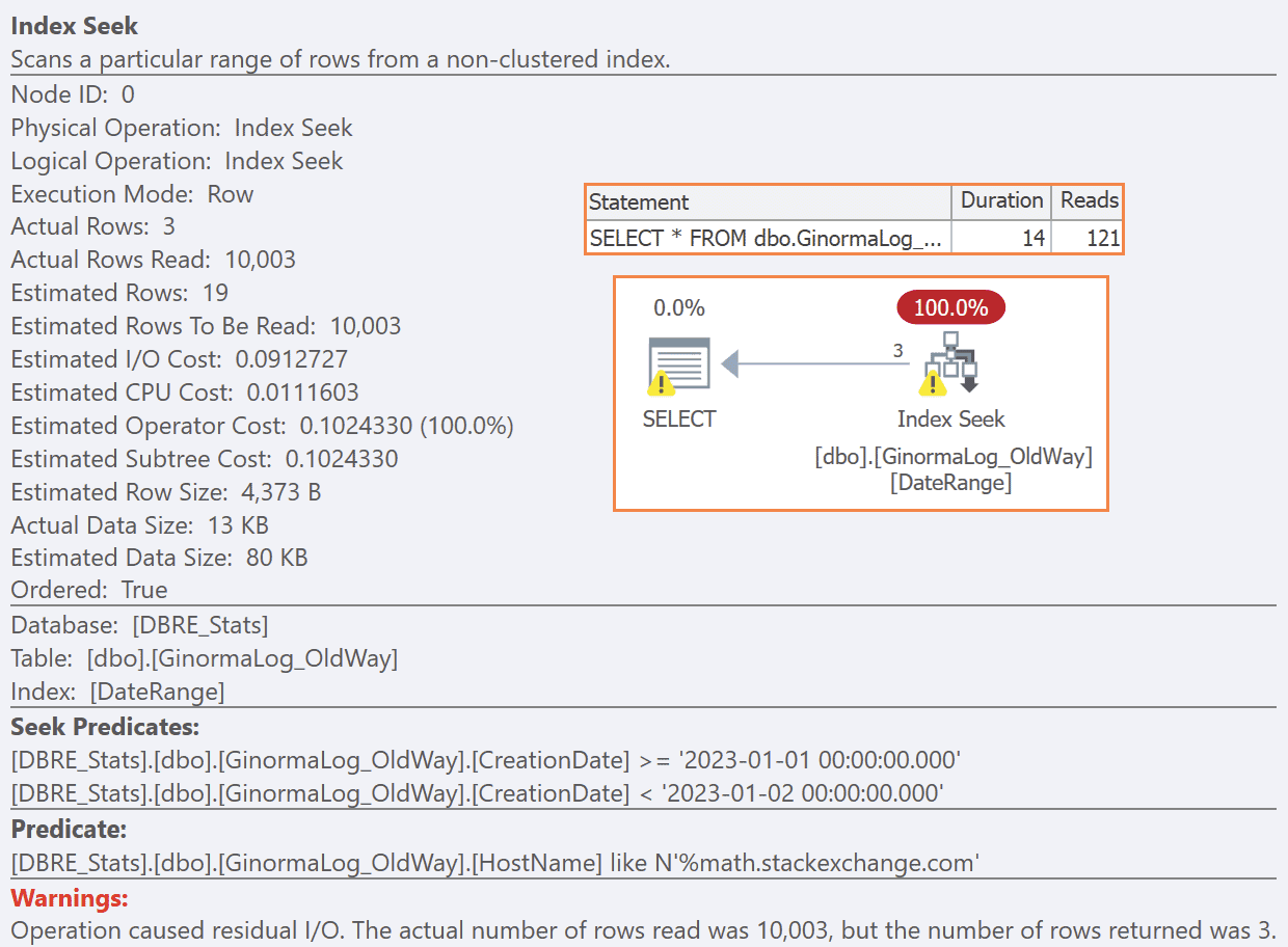
And sure enough, we get a plan that looks okay, especially in Management Studio – it has an index seek and everything! But that is misleading, because that index seek is doing a lot more work than it should. And in the real world, those reads and other costs are much higher, both because there are more rows to ignore, and every row is a lot wider:

So, then, what if we create an index on CreationDate, HostName?

CREATE INDEX Date_HostName
   ON dbo.GinormaLog_OldWay(CreationDate, HostName) 
   INCLUDE(Uri, QueryString);

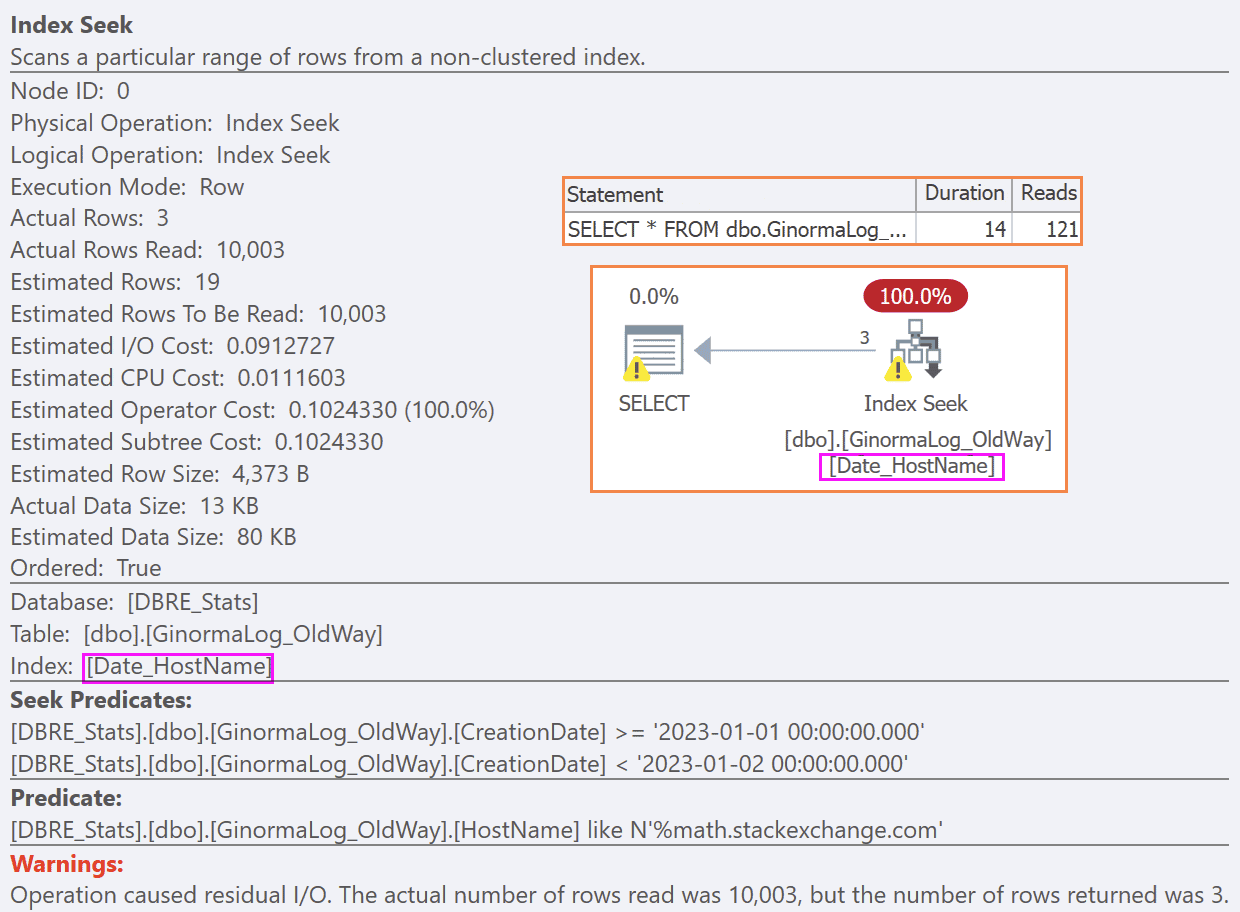
This doesn’t help. We still get the same plan, because whether or not the HostName shows up in the key, the bulk of the work is filtering the rows to the date range, and then checking the string is still just residual work against all the rows:

If we could coerce users to use more index-friendly queries without leading wildcards, like this, we may have more options:

WHERE CreationDate >= '20230101' 
   AND CreationDate <  '20230102'
   AND HostName IN 
   (
      N'math.stackexchange.com', 
      N'meta.math.stackexchange.com'
   );

In this case, you can see how an index (at least leading) on HostName might help:

CREATE INDEX HostName
   ON dbo.GinormaLog_OldWay(HostName, CreationDate) 
   INCLUDE(Uri, QueryString);

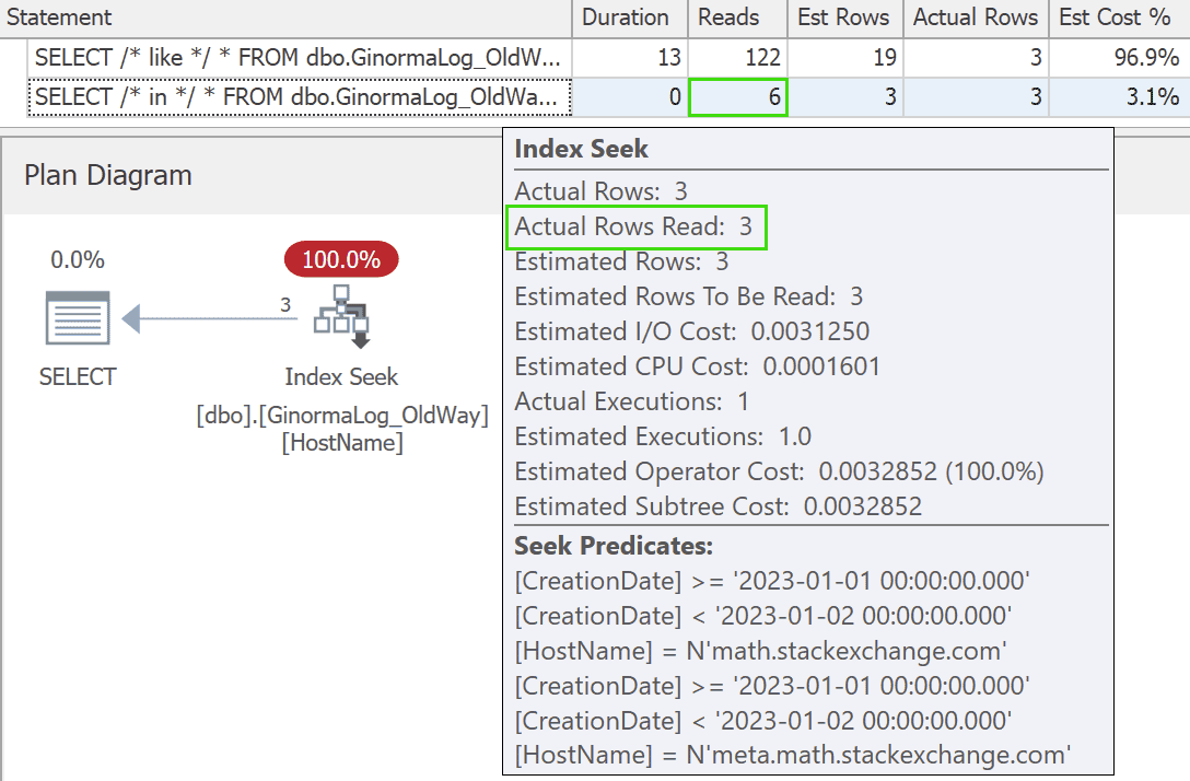
But this will only be effective if we can coerce users to change their habits. If they keep using LIKE, the query will still choose the older index (and results aren’t any better even if you force the new index). But with an index leading on HostName and a query that caters to that index, the results are drastically better:

This is not overly surprising, but I do empathize that it can be hard to persuade users to change their query habits and, even when you can, it can also be hard to justify creating additional indexes on already very large tables. This is especially true of log tables, which are write-heavy, append-only, and read-seldom.

When I can, I would rather focus on making those tables smaller in the first place.

Compression can help to an extent, and columnstore indexes, too (though they bring additional considerations). You may even be able to halve the size of this column by convincing your team that your host names don’t need to support Unicode.

For the adventurous, I recommend better normalization!

Think about it: If we log math.stackexchange.com a million times today, does it make sense to store 44 bytes, a million times? I would rather store that value in a lookup table once, the first time we see it, and then use a surrogate identifier that can be much smaller. In our case, since we know we won’t ever have over 32,000 Q&A sites, we can use smallint (2 bytes) – saving 22 bytes per row (or more, for longer host names). Picture this slightly different schema:

CREATE TABLE dbo.NormalizedHostNames
 (
   HostNameId smallint identity(1,1),
   HostName nvarchar(250) NOT NULL,
   CONSTRAINT PK_NormalizedHostNames PRIMARY KEY(HostNameId),
   CONSTRAINT UQ_NormalizedHostNames UNIQUE(HostName)
 );

 INSERT dbo.NormalizedHostNames(HostName)
 VALUES(N'math.stackexchange.com'),
       (N'meta.math.stackexchange.com'),
       (N'stackoverflow.com');

 CREATE TABLE dbo.GinormaLog_NewWay
 (
   Id           int identity(1,1) NOT NULL,
   HostNameId   smallint NOT NULL FOREIGN KEY 
                REFERENCES dbo.NormalizedHostNames(HostNameId),
   Uri          nvarchar(2048),
   QueryString  nvarchar(2048),
   CreationDate datetime,
   /* other columns */
   CONSTRAINT PK_GinormaLog_NewWay PRIMARY KEY(Id)
 );

 CREATE INDEX HostName
   ON dbo.GinormaLog_NewWay(HostNameId, CreationDate) 
   INCLUDE(Uri, QueryString);

Then the app maps the host name to its identifier (or inserts a row if it can’t find one), and inserts the id into the log table instead:

/* populate a few rows to search for (the needles) */

 INSERT dbo.GinormaLog_NewWay(HostNameId, Uri, QueryString, CreationDate)
 VALUES
   (1, N'/questions/show/', N'',            '20230101 01:24'),
   (1, N'/users/56789/',    N'?tab=active', '20230101 01:25'),
   (2, N'/q/98765/',        N'?x=124.54',   '20230101 01:26'); 
 GO

 /* put some realistic other traffic (the haystack) */

 INSERT dbo.GinormaLog_NewWay(HostNameId, Uri, QueryString, CreationDate)
 SELECT TOP (1000) 3, CONCAT(N'/q/', ABS(object_id % 10000)),
   CONCAT(N'?x=', name), DATEADD(minute, column_id, '20230101')
   FROM sys.all_columns;
 GO 10

 INSERT dbo.GinormaLog_NewWay(HostNameId, Uri, QueryString, CreationDate)
 SELECT TOP (1000) 3, CONCAT(N'/q/', ABS(object_id % 10000)),
   CONCAT(N'?x=', name), DATEADD(minute, -column_id, '20230125')
   FROM sys.all_columns;

First, let’s compare the sizes:

That’s a 36% reduction in space. When we’re talking about terabytes of data, this can drastically reduce storage costs and significantly extend the utility and lifetime of existing hardware.

What about our queries?

The queries are slightly more complicated, because now you have to perform a join:

SELECT * 
 FROM dbo.GinormaLog_NewWay AS nw
 INNER JOIN dbo.NormalizedHostNames AS hn
   ON nw.HostNameId = hn.HostNameId
 WHERE nw.CreationDate >= '20230101' 
   AND nw.CreationDate <  '20230102'
   AND hn.HostName LIKE N'%math.stackexchange.com';
   /* -- or 
   AND (hn.HostName IN (N'math.stackexchange.com',
        N'meta.math.stackexchange.com')); */

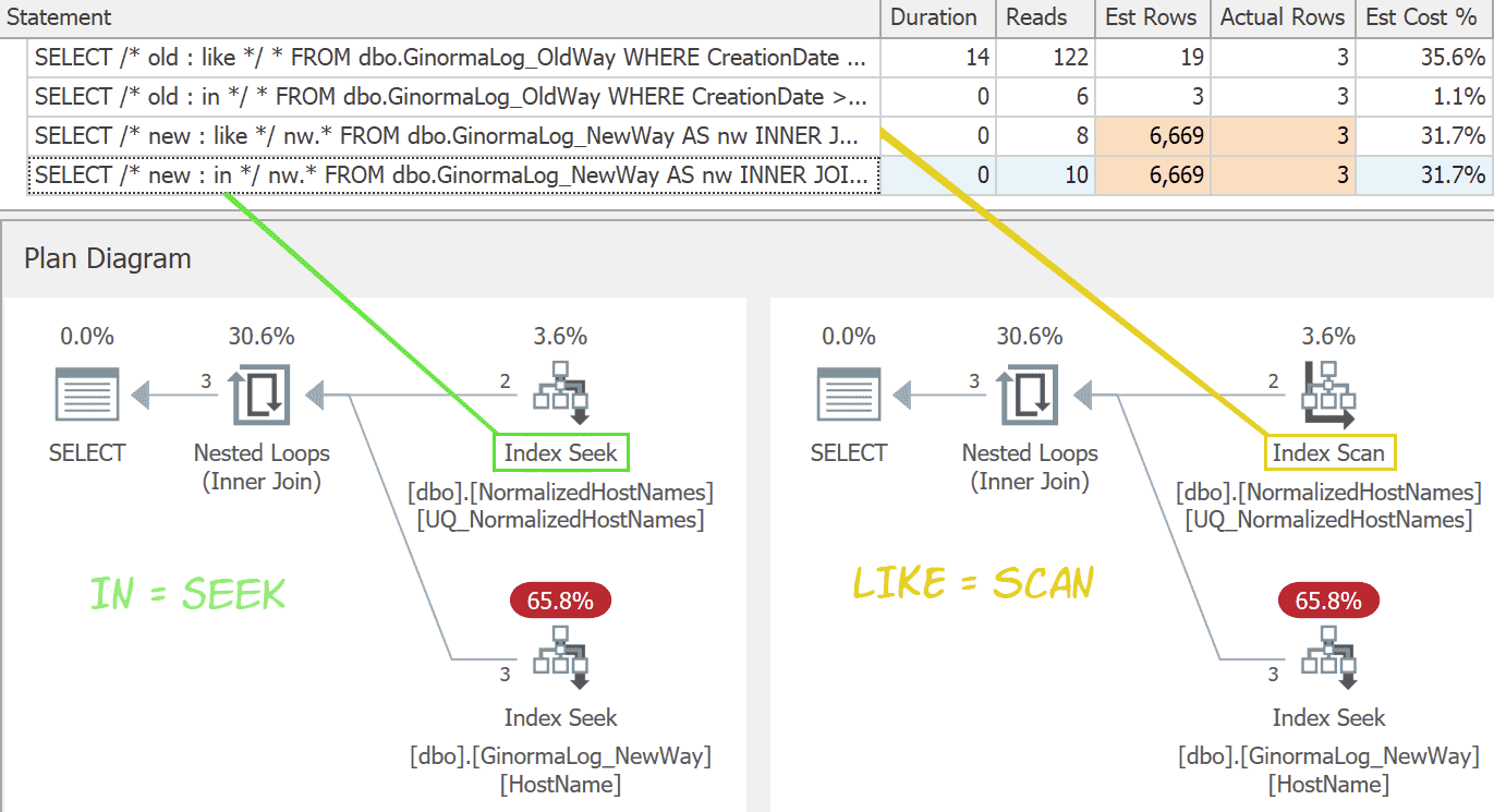
In this case, using LIKE isn’t a disadvantage unless the host names table becomes massive. The plans are almost identical, except that the LIKE variation can’t perform a seek. (Both are a little more horrible at estimates, but I don’t see how being any worse off the mark here will ever pick any other plan.)

This is one scenario where the difference between a seek and a scan is such a small part of the plan it is unlikely to be significant.

This strategy still requires analysts and other end users to change their query habits a little, since they need to add the join compared to when all of the information was in a single table. But you can make this change relatively transparent to them by offering views that simplify the joins away:

CREATE VIEW dbo.vGinormaLog
 AS
   SELECT nw.*, hn.HostName
   FROM dbo.GinormaLog_NewWay AS nw
   INNER JOIN dbo.NormalizedHostNames AS hn
     ON nw.HostNameId = hn.HostNameId;

Never use SELECT * in a view.

Querying the view, like this, still leads to the same efficient plans, and lets your users use almost exactly the same query they’re used to:

SELECT * FROM dbo.vGinormaLog
   WHERE CreationDate >= '20230101' 
     AND CreationDate <  '20230102'
     AND HostName LIKE N'%math.stackexchange.com';

Existing infrastructure vs. greenfield

Even scheduling the maintenance to change the way the app writes to the log table – never mind actually making the change – can be a challenge. This is especially difficult if logs are merely bulk inserted or come from multiple sources. It may be sensible to use a new table (perhaps with partitioning) and start adding new data going forward in a slightly different format, and leaving the old data as is, using a view to bridge them.

That could be complex, and I don’t mean to trivialize this change. I wanted to post this more as a “lessons learned” kind of thing – if you are building a system where you will be logging a lot of redundant string information, think about a more normalized design from the start. It’s much easier to build it this way now than to shoehorn it later… when it may well be too big and too late to change. Just be careful to not treat all potentially repeating strings as repeating enough to make normalization pay off. For host names at Stack Overflow, we have a predictably finite number, but I wouldn’t consider this for user agent strings or referrer URLs, for example, since that data is much more volatile and the number of unique values will be a large percentage of the entire set.

The post Normalize strings to optimize space and searches appeared first on Simple Talk.

from Simple Talk https://ift.tt/PTrgmWY
via

T-SQL Fundamentals: Controlling Duplicates

When people start learning a new field, for example T-SQL, it’s tempting to spend very little time trying to understand the fundamentals of the field so that you can quickly get to the advanced parts. You might think that you already understand what certain ideas, concepts and terms mean, so you don’t necessarily see the value in dwelling on them. That’s often the case with newcomers to T-SQL, especially because soon after you start learning the language, you can already write queries that return results, giving you a false impression that it’s a simple or easy language. However, without a good understanding of the foundations and roots of the language, you’re bound to end up writing code that doesn’t mean what you think it means. To be able to write robust and correct T-SQL code, you really want to spend a lot of energy on making sure that you have an in-depth understanding of the fundamentals.

A great example for a fundamental concept in T-SQL that seems simple but actually involves many subtleties is: duplicates. The concept of duplicates is at the heart of relational database design and T-SQL. Understanding what duplicates are is consequential to many of its features. It’s also important to understand the differences between how T-SQL handles duplicates versus how relational theory does.

In this article I focus on duplicates and how to control them. In order to understand duplicates correctly, you need to understand the concepts of distinctness and equality, which I’ll cover as well.

In my examples I will use the sample database TSQLV6. You can download the script file to create and populate this database and its ER diagram in a .ZIP file here. (You can find all of my downloads on my website at the following address: https://itziktsql.com/r-downloads)

What are duplicates in T-SQL?

T-SQL is a dialect of standard SQL So, the obvious place to look for the definition of duplicates is in the standard’s text, assuming you have access to it (you can purchase a copy using the link provided) and the stomach for it. If you do look for the definition of duplicates in the standard’s text, you’ll quickly start wondering how deep the rabbit hole goes.

Here’s the definition of duplicates in the standard:

Duplicates

Two or more members of a multiset that are not distinct

So now you need to figure out what multiset and distinct mean.

Let’s start with multiset. This can get a bit confusing since there’s both a mathematical concept called multiset and a specific feature in the SQL standard called MULTISET (one of two kinds of collection types: ARRAY and MULTISET). T-SQL doesn’t support the standard collection types ARRAY and MULTISET. However, the mathematical concept of a multiset is quite important to understand for T-SQL practitioners.

Here’s the description of a multiset from Wikipedia:

Multiset

In mathematics, a multiset (or bag, or mset) is a modification of the concept of a set that, unlike a set, allows for multiple instances for each of its elements.

In other words, whereas a set is a collection of distinct elements, a multiset allows duplicates. Oops…

I’m not sure why they chose in the standard to define duplicates via multisets. To me, it should be the other way around. I think that it’s sufficient to understand the concept of duplicates via distinctness alone, and later talk about what multisets are.

So, back to the definitions section in the SQL standard, here’s the definition of distinctness:

Distinct (of a pair of comparable values)

Capable of being distinguished within a given context.

Hmm… not very helpful. But wait, there’s more! There’s NOTE 8:

NOTE 8 — Informally, two values are distinct if neither is null and the values are not equal. A null value and a nonnull value are distinct. Two null values are not distinct. See Subclause 4.1.5, “Properties of distinct”, and the General Rules of Subclause 8.15, “<distinct predicate>”.

Let’s start with the meaning of a given context. This has to do with the contexts in SQL where a pair of values can be compared. It could be a query filter, a join predicate, a set operator, the DISTINCT set quantifier in the SELECT list or an aggregate function, grouping, uniqueness, and so on.

Next, let’s talk about the meaning of a pair of comparable values. The concept of distinctness is relevant to a pair of values that can be compared. Later the standard contrasts this with values of a user-defined type that has no comparison type, in which case distinctness is undefined.

I also need to mention here that when the standard uses the term value, it actually includes both non-NULL values and NULLs. To some, myself included, a NULL is a marker for a missing value, and therefore the term NULL value is actually incorrect. But what could be an inclusive term for both NULLs and non-NULL values? I don’t know that there’s a common industry term that is simple, intuitive and accurate. If you know one, let me know! Since our focus is things that can be compared, maybe we’ll just use the term comparands. And by the way, in SQL, the concepts of duplicates and distinctness are of course relevant not just to scalar comparands, but also to row comparands.

What’s left to understand is what capable of being distinguished means. Note 8 goes into details trying to explain distinctness via equality, with exceptions when NULLs are involved. And as usual, it sends you elsewhere to read about properties of distinct, and the distinct predicate.

What’s crucial to understand here is that there’s an important difference between equality-based comparison (or inequality) and distinctness-based comparison in SQL. You understand the difference using predicate logic. Given comparands c1 and c2, here are the truth values for the inequality-based predicate c1 <> c2 versus the distinctness-based counterpart c1 is distinct from c2:

c1	c2	c1 <> c2	c1 is distinct from c2
non-NULL X	non-NULL X	false	false
non-NULL X	non-NULL Y	true	true
any non-NULL	NULL	unknown	true
NULL	any non-NULL	unknown	true
NULL	NULL	unknown	false

As you can see, with inequality, when both comparands are non-NULL, if they are the same the comparison evaluates to false and if they are different it evaluates to true. If any of the comparands is NULL, including both, the comparison evaluates to the truth value unknown.

With distinctness, when both comparands are non-NULL, the behavior is the same as with inequality. When you have NULLs involved, they are basically treated just like non-NULL values. Meaning that when both comparands are NULL, IS DISTINCT FROM evaluates to false, otherwise to true.

Similarly, given comparands c1 and c2, here are the truth values for the equality-based predicate c1 = c2 versus the distinctness-based counterpart c1 is not distinct from c2:

c1	c2	c1 = c2	c1 is not distinct from c2
non-NULL X	non-NULL X	true	true
non-NULL X	non-NULL Y	false	false
any non-NULL	NULL	unknown	false
NULL	any non-NULL	unknown	false
NULL	NULL	unknown	true

As you can see, with equality, when both comparands are non-NULL, if they are the same the comparison evaluates to true and if they are different it evaluates to false. If any of the comparands is NULL, including both, the comparison evaluates to the truth value unknown.

With non-distinctness, when both comparands are non-NULL, the behavior is the same as with equality. When you have NULLs involved, they are basically treated just like non-NULL values. Meaning that when both comparands are NULL, IS NOT DISTINCT FROM evaluates to true, otherwise to false.

In case you’re not already aware of this, starting with SQL Server 2022, T-SQL supports the explicit form of the standard distinct predicate, using the syntax <comparand 1> IS [NOT] DISTINCT FROM <comparand 2>. You can find the details here.

As you can gather, trying to understand things from the standard can be quite an adventure.

So let’s try to simplify our understanding of duplicates.

First, you need to understand the concept of distinctness. This is done using predicate logic by understanding the difference between equality-based comparison and distinctness-based comparison, and familiarity with the distinct predicate and its rules.

These concepts are not trivial to digest for the uninitiated, but they are critical for a correct understanding of the concept of duplicates.

Assuming you have the concept of distinctness figured out, you can then understand duplicates.

Duplicates

Comparands c1 and c2 are duplicates if c1 is not distinct from c2. That is, if the predicate c1 IS NOT DISTINCT FROM c2 evaluates to true.

The comparands c1 and c2 can be scalar comparands, in contexts like filter and join predicates, or row comparands, in contexts like the DISTINCT quantifier in the SELECT list and set operators.

T-SQL/SQL Versus Relational Theory

Even though standard SQL and the T-SQL dialect, which is based on it, are founded in relational theory, they deviate from it in a number of ways, one of which is the handling of duplicates. The main structure in relational theory is a relation. Relational expressions operate on relations as inputs and emit a relation as output.

The counterpart to a relation is a table in SQL. Similar to relational expressions, table expressions, such as ones defined by queries, operate on tables as inputs and emit a table as output.

A relation has a heading and a body. The heading of a relation is a set of attributes. Similarly, the heading of a Table is a set of columns. There are interesting differences between the two, but that’s not the focus of this article.

The body of a relation is a set of tuples. Recall that a set has no duplicates. This means that by definition, a relation must have at least one candidate key.

Unlike the body of a relation, the body of a table is a multiset of rows. Recall, a multiset is similar to a set, only it does allow duplicates. Indeed, you don’t have to define a key in a table (no primary key or unique constraint), and if you don’t, the table can have duplicate rows.

Furthermore, even if you do have a key defined in a table; unlike a relational expression, a table expression that is based on a base table with a key, does not by default eliminate duplicates from the result table that it emits.

Suppose that you need to project the countries where you have employees. In relational theory you formulate a relational expression doing so, and you don’t need to be explicit about the fact that you don’t want duplicate countries in the result. This is implied from the fact that the outcome of a relational expression is a relation. Suppose you try achieving the same in T-SQL using the following table expression:

SELECT country FROM HR.Employees

As an aside, you might be wondering now why I didn’t terminate this expression, despite the fact that I keep telling people how important it is to terminate all statements in T-SQL as a best practice. Well, you terminate statements in T-SQL. Statements do something. My focus now is the table expression returning a table with the cities where you have employees. The expression is the query part without the terminator, and is the part that can be nested in more elaborate table expressions.

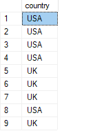
Back to our discussion about duplicates. Despite the fact that the underlying Employees table has a key and hence no duplicates, this table expression which is based on Employees, does have duplicates in its table result:

Run the following code:

USE TSQLV6;

SELECT country FROM HR.Employees;

You get the following output:

Of course, T-SQL does give you tools to eliminate duplicates in a table expression if you want to, it’s just that in some cases it doesn’t do so by default. In the above example, as you know well, you can use the DISTINCT set quantifier for this purpose. People often learn a dialect of SQL like T-SQL without learning the theory behind it. Many are so used to the fact that returning duplicates is the default behavior, that they don’t realize that that’s not really normal in the underlying theory.

Controlling duplicates in T-SQL/SQL

If I tried covering all aspects of controlling duplicates in T-SQL, I’d probably easily end up with dozens of pages. To make this article more approachable, I’ll focus on features that involve using quantifiers to allow or restrict duplicates.

SELECT List

T-SQL allows you to apply a set quantifier ALL | DISTINCT to the SELECT list of a query. The default is ALL if you don’t specify a quantifier.

The earlier query returning the countries where you have employees, without removal of duplicates, is equivalent to the following:

SELECT ALL country FROM HR.Employees;

As you know, you need to explicitly use the DISTINCT quantifier to remove duplicates, like so:

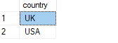
SELECT DISTINCT country FROM HR.Employees;

This code returns the following output:

Aggregate Functions

Similar to the SELECT list’s quantifier, you can apply a set quantifier ALL | DISTINCT to the input of an aggregate function. Also here the ALL quantifier is the default if you don’t specify one explicitly. With the ALL quantifier—whether explicit or implied—redundant duplicates are retained. The following two queries are logically equivalent:

SELECT COUNT(country) AS cnt FROM HR.Employees;

SELECT COUNT(ALL country) AS cnt FROM HR.Employees;

Both queries return a count of 9 since there are nine rows where country is not NULL.

Again, you can use the DISTINCT quantifier if you want to remove redundant duplicates, like so:

SELECT COUNT(DISTINCT country) AS cnt FROM HR.Employees;

This query returns 2 since there are two distinct countries where you have employees.

Note that at the time of writing, T-SQL supports the DISTINCT quantifier with grouped aggregate functions, but not with windowed aggregate functions. There are workarounds, but they are far from being trivial.

Set operators

Set operators allow you to combine data from two input table expressions. The SQL standard supports three set operators UNION, INTERSECT and EXCEPT, each with two possible quantifiers ALL | DISTINCT. With set operators the DISTINCT quantifier is the default if you don’t specify one explicitly.

At the time of writing, T-SQL supports only a subset of the standard set operators. It supports UNION (implied DISTINCT), UNION ALL, INTERSECT (implied DISTINCT) and EXCEPT (implied DISTINCT). It doesn’t allow you to be explicit with the DISTINCT quantifier, although that’s the behavior that you get by default, and it supports the ALL option only with the UNION ALL operator. It currently does not support the INTERSECT ALL and EXPECT ALL operators. I’ll explain all standard variants, and for the missing ones in T-SQL, I’ll provide workarounds.

You apply a set operator to two input table expressions, which I’ll refer to as TE1 and TE2:

TE1
<set operator> 
TE2

The above represents a table expression.

A statement based on a table expression with a set operator can have an optional ORDER BY clause applied to the result, using the following syntax:

TE1 <set operator>  TE2 
[ORDER BY <order by list>];

You’re probably familiar with the set operators that T-SQL supports. Still, let me briefly explain what each operator does:

• UNION: Returns distinct rows that appear in TE1, TE2 or both. That is, if row R appears in TE1, TE2 or both, irrespective of number of occurrences, it appears exactly once in the result.
• UNION ALL: Returns all rows that appear in TE1, TE2 or both. That is, if row R appears m times in TE1 and n times in TE2, it appears m + n times in the result.
• INTERSECT: Returns distinct rows that are common to both TE1 and TE2. That is, if row R appears at least once in TE1, and at least once in TE2, it appears exactly once in the result.
• INTERSECT ALL: Returns all rows that are common to both TE1 and TE2. That is, if row R appears m times in TE1 and n times in TE2, it appears minimum(m, n) times in the result. For example, if R appears 5 times in TE1 and 3 times in TE2, it appears 3 times in the result.
• EXCEPT: Returns distinct rows that appear in TE1 but not in TE2. That is, if a row R appears in TE1, irrespective of the number of occurrences, and does not appear in TE2, it appears exactly once in the output.
• EXCEPT ALL: Returns all rows that appear in TE1 but don’t have an occurrence match in TE2. That is, if a row R appears m times in TE1, and n times in TE2, it appears maximum((m - n), 0) times in the result. For example, if R appears 5 times in TE1 and 3 times in TE2, it appears 2 times in the result. If R appears 3 times in TE1 and 5 times in TE2, it doesn’t appear in the result.

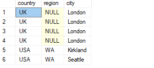
An interesting question is why would you use a set operator to handle a given task as opposed to alternative tools to combine data from multiple tables, such as joins and subqueries? To me, one of the main benefits is the fact that when set operators compare rows, they implicitly use distinctness-based comparison and not equality-based comparison. Recall that distinctness-based comparison handles NULLs and non-NULL values the same way, essentially using two-valued logic instead of three-valued logic. That’s often the desired behavior, and with set operators it simplifies the code a great deal. For example, the following code identifies distinct locations that are both customer locations and employee locations:

SELECT country, region, city FROM Sales.Customers
INTERSECT
SELECT country, region, city FROM HR.Employees;

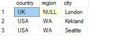
This code generates the following output:

Since set operators implicitly use the distinct predicate to compare rows (not to confuse with the fact that without an explicit quantifier they use the DISTINCT quantifier by default), you didn’t need to do anything special to get a match when comparing two NULLs and a nonmatch when comparing a NULL with a non-NULL value. The location UK, NULL, London is part of the result since it appears in both inputs.

Also, with no explicit quantifier specified, a set operator uses an implicit DISTINCT quantifier by default. Remember that with INTERSECT, as long as at least one occurrence of a row appears in both sides, INTERSECT returns one occurrence of the row in the result.

As an exercise, I urge you to write a logically equivalent solution to the above code, using either joins or subqueries. Of course it’s doable, but not this concisely.

As mentioned, the standard also supports an ALL version of INTERSECT. For example, the following standard query returns all occurrences of locations that are both customer locations and employee locations (don’t run it against SQL Server since it’s not supported in T-SQL):

SELECT country, region, city FROM Sales.Customers
INTERSECT ALL
SELECT country, region, city FROM HR.Employees;

If you want to use a solution that is supported in T-SQL, the trick is to compute row numbers in each input table expression to number the duplicates, and then apply the operation to the inputs including the row numbers. You can then exclude the row numbers from the result by using a named table expression like a CTE. Here’s the complete code:

WITH C AS
(
  SELECT country, region, city, 
    ROW_NUMBER() OVER(PARTITION BY country, region, city 
                              ORDER BY (SELECT NULL)) AS rownum
  FROM Sales.Customers
  
  INTERSECT
  
  SELECT country, region, city, 
    ROW_NUMBER() OVER(PARTITION BY country, region, city 
                              ORDER BY (SELECT NULL)) AS rownum
  FROM HR.Employees
)
SELECT country, region, city
FROM C;

This code generates the following output:

The location UK, NULL, London appears 6 times in the first input table expression and 4 times in the second, therefore 4 occurrences intersect.

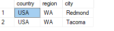
You can handle an except need very similarly. If you’re interested in an except distinct operation, you use the EXCEPT (implied DISTINCT) in T-SQL. For example, the following code returns distinct employee locations that are not customer locations:

SELECT country, region, city FROM HR.Employees
EXCEPT
SELECT country, region, city FROM Sales.Customers;

This code generates the following output:

If you wanted all employee locations that per occurrence don’t have a matching customer location, the standard code for this looks like so:

SELECT country, region, city FROM HR.Employees
EXCEPT ALL
SELECT country, region, city FROM Sales.Customers;

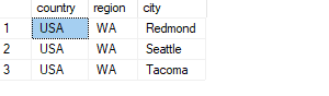
However, T-SQL doesn’t support the ALL quantifier with the EXCEPT operator. You can use a similar trick to the one you used to achieve the equivalent of INTERSECT ALL. You can achieve the equivalent of EXCEPT ALL by applying EXCEPT (implied DISTINCT) to inputs that include row numbers that number duplicate, like so:

WITH C AS
(
  SELECT country, region, city, 
    ROW_NUMBER() OVER(PARTITION BY country, region, city 
                            ORDER BY (SELECT NULL)) AS rownum
  FROM HR.Employees
  
  EXCEPT
  
  SELECT country, region, city, 
    ROW_NUMBER() OVER(PARTITION BY country, region, city 
                            ORDER BY (SELECT NULL)) AS rownum
  FROM Sales.Customers
)
SELECT country, region, city
FROM C;

This code generates the following output:

Curiously, Seattle appears once in this result of except all but didn’t appear at all in the result of the except distinct version. You might initially think that there’s a bug in the code. But think carefully what could explain this? There are two employees from Seattle and one customer from Seattle. The except distinct operation isn’t supposed to return any occurrences in the result, yet the except all operation is indeed supposed to return one occurrence.

Conclusion

Without proper understanding of the foundations of T-SQL—primarily relational theory and its own roots—it’s hard to truly understand what you’re dealing with. In this article I focused on duplicates. A concept that to most seems trivial and intuitive. However, as it turns out, a true understanding of duplicates in T-SQL is far from being trivial.

You need to understand the differences between how relational theory treats duplicates versus SQL/T-SQL. A relation’s body doesn’t have duplicates whereas a table’s body can have those.

It’s very important to understand the difference between distinctness-based comparison, such as when using the distinct predicate explicitly or implicitly, versus equality-based comparison. Then you realize that in T-SQL, two comparands are duplicates when one is not distinct from the other.

You also need to understand the nuances of how T-SQL handles duplicates, the cases where it retains redundant ones versus cases where it removes those. You also need to understand the tools that you have to change the default behavior using quantifiers such as DISTINCT and ALL.

I discussed controlling duplicates in a query’s SELECT list, aggregate functions and set operators. But there are other language elements where you might need to control them such as handling ties with the TOP filter, window functions, and others.

What I hope that you take away from this article is the significance of investing time and energy in learning the fundamentals. And if you haven’t had enough of T-SQL Fundamentals, and I’m allowed a shameless plug, check out my new book T-SQL Fundamentals 4th Edition.

May the 4th be with you!

 

The post T-SQL Fundamentals: Controlling Duplicates appeared first on Simple Talk.

from Simple Talk https://ift.tt/zn5NIH8
via

Microsoft Fabric and the Delta Tables Secrets

Microsoft Fabric storage uses OneLake and Delta Tables, the core storage of all Fabric objects, as explained in my introduction to Microsoft Fabric.

Either if you use lakehouses, data warehouses, or even datasets, all the data is stored in the OneLake. OneLake uses Delta Tables as storage. In this way, we need to be aware of some “secrets” related to delta table storage in order to make the best decisions possible for our data platform solution.

Let’s analyze some of the Parquet and Delta Table behaviors.

Parquet and Delta

Parquet is an open source format which became famous as one of the most used formats in data lakes. It’s a columnar storage format intended to store historical data.

One very important “secret”, and the main subject of this blog is: Parquet format is immutable. It’s not possible to change the content of a Parquet file. It’s intended for historical data.

Although the main objective is for historical data, many people and companies worked on this problem. The result was Delta Tables.

Delta Tables use the Parquet format, it’s not a different format. The immutable behavior continues. However, Delta Tables use an additional folder as a transaction log. The operations are registered in the delta logs, marking records with updates and deletes.

In this way, the underlying immutable behavior is still present, but we can work with the data in a transactional way, allowing updates and deletes, for example.

Time Travel

The delta logs allow us to make what’s called Time Travel. We can retrieve the information from a delta table in the way it was on a specific date and time, as long as the logs are kept complete.

The access to the entire historical of data changes is an important resource for a data storage.

Data Modelling

The need to keep historical data is way older than technologies such as Delta Time Travel, which allow us to keep them. The Data Modelling techniques, such as Data Warehouse modelling, proposed solutions for historical storage a long time ago.

One of the features used for this purpose is called Slowly Changing Dimensions, or Dimension Type 2. When we design a start schema, we decide which dimensions should keep an entire history and which ones aren’t worth the trouble and a simple update on the records would be enough.

For example, let’s consider a dimension called Customer. If we decide to keep the dimension as a SCD dimension, every time a customer record is changed in production, we create a new version of the record in the intelligence storage (data warehouse, data lake, whatever the name).

On the other hand, if we decide that a dimension is not worth keeping a history, we can just update the record in the intelligence storage when needed.

The decision of using a SCD dimension or not, and many more, are all made during modelling. They are independent of any technical feature capable of keeping the history of the data. The history is designed during modelling and kept by us.

Choosing Between Time Travel and Data Modelling

We have the possibility to use data modelling to control the history of our storage, or use the technical features, such as Time Travel.

This leads to several possibilities with different consequences:

Approach	Possible Results
We can choose to rely on time travel for the entire history storage of our data	This will tie the history of your data solution with a specific technological feature. It also creates the risk of performance issues related to executing updates in a delta table. Let’s talk more in depth about the technology and leave the decision to you.
We can choose to rely on the modelling for the entire history and not depend on the time travel feature	This creates additional modelling and ingestion work, plus additional work to avoid performance issues with the delta log. The work to avoid performance issues with the delta log may be easier than if we were really relying on it.

The decision whether we should rely on modelling, on technology or stay somewhere in the middle is complex enough to generate many books. What’s important on this blog is to understand the decision is present when designing an architecture with Microsoft Fabric.

In order to make a well-informed decision, we need to understand how the delta tables process updates/deletes.

Lakehouse Example

The example will be made using a table called Fact_Sale. You can use a pipeline to import the data from https://ift.tt/bJBmN0R to the files area of one Fabric Lakehouse. The article about Lakehouse and ETL explains how to build a pipeline to bring data to the Files area.

The article https://www.red-gate.com/simple-talk/blogs/microsoft-fabric-using-notebooks-and-table-partitioning-to-convert-files-to-tables/ explains this import process and how we can partition the data by Year and Quarter, making a more interesting example. The notebook code to import the partitioned data to the Tables area of the lakehouse is the following:

from pyspark.sql.functions import col, year, month, quarter
table_name = 'fact_sale'
df = spark.read.format("parquet").load('Files/fact_sale_1y_full')
df = df.withColumn('Year', year(col("InvoiceDateKey")))
df = df.withColumn('Quarter', quarter(col("InvoiceDateKey")))
df = df.withColumn('Month', month(col("InvoiceDateKey")))
df.write.mode("overwrite").format("delta").partitionBy("Year","Quarter").save("Tables/" + table_name)

The default size for a Parquet file in the Fabric environment is 1GB (1073741824 bytes). This is defined by the session configuration spark.microsoft.delta.optimizeWrite.binSize and has the purpose to avoid the delta lake small files problem. Although this is a common problem, the writing on delta tables can cause consequences when the file is too big. Let’s analyze this as well.

You can find more about Spark configuration on this blog and more about the small files problem on this link.

On our example, this configuration generated a single parquet file for each quarter, this will help to identify what’s happening during the example.

The Data we Have

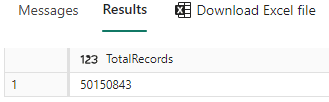
We need to identify the total of records we have, the total records for each quarter, and the minimum and maximum SalesKey value in each quarter in order to build the example.

We can use the SQL Endpoint to run the following queries:

SELECT Count(*) AS TotalRecords
FROM   fact_sale 

SELECT quarter,
       Count(*)     SalesCount,
       Min(salekey) MinKey,
       Max(salekey) MaxKey
FROM   fact_sale
GROUP  BY quarter 

Test query and Execution Time

For test purposes, let’s use the following query:

SELECT customerkey,
       Sum(totalincludingtax) TotalIncludingTax
FROM   fact_sale
GROUP  BY customerkey 

This query makes a grouping on all our records by CustomerKey, across the quarter partitions, creating a total of Sales by customer. On each test, I will execute this query 10 times and check the initial, minimum, and maximum execution time.

 

First 10 Executions
Initial	2.639 seconds
Minimum	1.746 seconds
Maximum	3.32 seconds
Average	2.292 seconds

Updating one single record

As the first test, let’s update one single sales record in each quarter. We will use a notebook to execute the following code:

%%sql
update fact_sale set TotalIncludingTax=TotalIncludingTax * 2
where SaleKey = 6000000;

update fact_sale set TotalIncludingTax=TotalIncludingTax * 2
where SaleKey = 15624569 ;

update fact_sale set TotalIncludingTax=TotalIncludingTax * 2
where SaleKey = 35270205;

update fact_sale set TotalIncludingTax=TotalIncludingTax * 2
where SaleKey = 45032105;

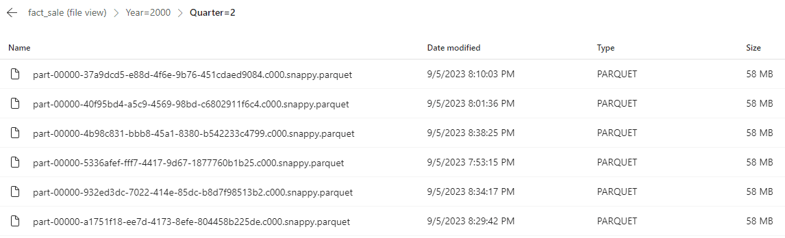
After executing these updates, if you look on the table Parquet files, you will notice each parquet file containing the record updated was duplicated.

The parquet file continues to be immutable, in order to update a record, the entire file is duplicated with the record update and the delta logs register this update.

In our example, we updated 4 records, but each one was in a different parquet file. As a result, all the parquet files were duplicated (one for each quarter).

Remember the default file size is 1GB. A single record update will result in the duplication of a 1GB file. The big file size may have a bad side effect if you decide to use upserts or deletes too much.

Testing the Execution

Let’s test the execution of our sample query again and get the number after these duplication of parquet files:

After Updating 1 record
Initial	6.692 seconds
Minimum	1.564 seconds
Maximum	3.166 seconds (ignoring initial)
Average	2.8955 seconds
Average Ignoring Initial	2.4374 seconds

There is a initial execution substantially slower and the average, even ignoring the initial execution, is slower, but not much.

Updating many records

Let’s change a bit the script and update a higher volume of records each quarter. You can execute the script below many times and each time you execute you will see the parquet files being duplicated.

%%sql
update fact_sale set TotalIncludingTax=TotalIncludingTax * 2
where SaleKey < 7000000;

update fact_sale set TotalIncludingTax=TotalIncludingTax * 2
where SaleKey > 14624564 AND SaleKey < 18624564;

update fact_sale set TotalIncludingTax=TotalIncludingTax * 2
where SaleKey > 28270201 AND SaleKey < 35270201;

update fact_sale set TotalIncludingTax=TotalIncludingTax * 2
where SaleKey > 42032102 AND SaleKey < 45032102;

Result

After executing the update script 4 times, we end up with 6 files on each partition. The original file, the file created by the update of a single record and the 4 files created when updating multiple record.

These are the results of the test query execution:

After Updating 1 record
Initial	11.894 seconds
Minimum	1.553 seconds
Maximum	2.286 seconds (ignoring initial)
Average	2.9394 seconds
Average Ignoring Initial	1.9494 seconds

The test seems to illustrate only the initial query is affected and affected a lot. After the data is in cache, the files in the delta table don’t affect the query, or at least, it seems so.

On one hand, this illustrates the problem. On the other hand, we are talking about a few seconds difference for a set of 50 million records.

Cleaning the Table

The process of cleaning the table from unlinked parquet files is executed by the statement VACUUM. There are some important points to highlight about this process:

• If you decide to manage yourself the data history using data modelling, this needs to be a regular process on tables affected by updates and deletes.
• On the other hand, if you decide to use Time Travel to manage history, you can’t execute this process, otherwise you will lose the time travel capability.

This process needs to be executed very carefully. You can’t try to delete files while you have some process in execution over the data. You need to ensure this will only be executed while you don’t have anything running over the data.

The default method to ensure this is to only delete files older than one specific time. For example, if you want to delete unlinked files younger than 168 hours, you need to activate a special spark session configuration to ensure you are aware about what you are doing.

In this way, the example below, which activates this configuration and executes the VACUUM with 0 retention, is only for test purposes, not for production scenarios.

spark.conf.set("spark.databricks.delta.retentionDurationCheck.enabled", "false")

 

 

%%sql
VACUUM 'Tables/fact_sale' RETAIN 0 HOURS

After executing this cleaning, the additional files will disappear and only the most updated will remain.

Onelake is for all

This process affects not only the lakehouse, but the data warehouse as well. In the lakehouse, the SQL Endpoint is read-only, but the Data Warehouse is read-write with MERGE operations.

Conclusion

Microsoft Fabric is a PaaS environment for the entire Enterprise Data Architecture and capable of enabling the most modern architectures, such as Data Mesh.

However, we should never lose track of the data concepts, such as the fact the data intelligence storage is intended to be read-only and for historical purposes. Our architectural decisions may have an impact on the result which may not be so obvious in a PaaS environment.

The post Microsoft Fabric and the Delta Tables Secrets appeared first on Simple Talk.

from Simple Talk https://ift.tt/a9T8A5N
via