Monday, January 31, 2022

Saving and Sharing Log Analytics Query

Log Analytics uses KQL – Kusto Query Language – as the query language for the log storage. On the past, we could only save the queries  in the Log Analytics Workspace and it was not easy to share them

The new feature to change this scenario is the Log Analytics Query Pack. This feature is an object capable to contain the queries we would like to save. Log Analytics Workspace can read the queries in the query pack.

This feature is still in preview. Some details will seem to be incomplete, but there is no doubt this is an important feature

Default Query Pack

If you ignore the query packs, the query packs will ignore you. Log Analytics creates the default query pack automatically the first time you save a query. This will happen for each subscription.

Saving Queries

When you build a query you can Save a query or a function, the process is slightly different. The functions can be saved only in the workspace, not in a query pack. Let’s keep the focus on the query.

When you build a query you can save it to a query pack. You have the option to save on the default query pack or choose a query pack to save it.

If we are saving the query to the default query pack the entire process can be transparent. We save the query and all workspaces on the same subscription are able to see the query.

On the other hand, if we are using custom query packs we should use the Tags carefully, so we will be able to find the queries easily on the Logs UI.

There are 3 types of Tags we can use on our queries, they are:

Category: The Category Tag is also used by the example queries provided by Microsoft to classify the purpose of the query. We can fit the query in the existing categories or create our own.

Resource Type: The idea of this tag is to classify the queries by the type of resource they are using. However, my recommendation is to use this tag to classify the queries by Query Pack in which it’s saved. The UI doesn’t provide in a very good way the information about the source query pack. It’s up to us to use the Tag fields to classify by query pack.

Label: This is a more “open” Tag field, you can use this for many different purposes. However, this field is not included (at least not yet) in the Filter or Group By UI options explained further on this blog. Due to this, I don’t recommend the use of the Label to classify by query pack.

Reading Queries

The Logs UI, when we select the option on a Log Analytics Worskpace, show us two windows: One popup window, displayed first, allowing us to select a query to edit or execute, it’s like an introduction window; The main query building window, which will display existing queries and allow us to build new ones.

On the popup window, a new option was included allowing us to select the query packs we would like to see on the query editor. The Log Analytics Workspace will remember our selection, so usually we may need to make this selection once, unless the need of additional queries or functions appear.

On the UI, after selecting the query packs, you can close this window and even so your selection will still be remembered.

On the main query editor window, the information about the query pack is displayed only in two different places:

Group by option: The Group by option to group the queries has the option to group the queries by the query type. There are two main query types: “Example Query”, the examples provided by Microsoft and “Query Pack” queries, the queries saved in query packs, either the default or custom ones.

This option can tell you what queries are from query packs, but it doesn’t break down the queries by query pack. In order to achieve this you would need to use the Tag together the group by, as explained before.

Query Popup: Each query has a popup window displayed when we select the query. This popup window tell us the source of the query. It’s useful for individual queries, but to find the queries from one query pack, for example, we would need to look query by query. We avoid that using the Tag to Filter or Group the queries by query pack, as mentioned before.

Summary

Log Analytics is a very important feature on Azure and can be used even for on premises implementations. The Query Packs expand the possibility to create reusable KQL queries and spread Log Analytics culture on an enterprise level

References

The post Saving and Sharing Log Analytics Query appeared first on Simple Talk.


from Simple Talk https://ift.tt/9Cj1Xzd3t
via

Wednesday, January 26, 2022

DBAs and DevOps

Lately, you’ve heard about DevOps. Is it just another buzzword, or is it something you should investigate?

DevOps emerged over ten years ago to solve the problems of the Agile methodology. Not that Agile is bad, but there were often disconnects between developers and the operation teams who had to deploy the software. Software that “worked on my laptop” often failed when deployed.

DevOps is

The union of people, process, and products to enable continuous delivery of value to our end users –Donovan Brown, Partner Program Manager, Azure Incubations at Microsoft

There are other definitions, but I like this one because the people and process are just as important as the products (tools). There are no prescribed techniques or tools in this definition, and each organization must figure out what works best for them. DevOps works by delivering small incremental changes quickly, removing bottlenecks, and automating everything, including infrastructure for development, builds, testing, quality assurance, etc.

DBAs tend to use automation to avoid performing repetitive tasks like installations, backups, and other maintenance manually. (I typically would write a script if I needed to do something at least three times.) DevOps, however, takes automation to a whole other level. According to the Accelerate State of DevOps 2021 report, most Elite performers deploy changes multiple times per day on demand. Frequent, small changes are less likely to require hotfixes than large, infrequent ones, but this seems counterintuitive when thinking about databases.

App development lends itself easily to DevOps because it’s easy to replace files or services and roll back to an earlier version or servers with the earlier version, if necessary. However, you usually cannot do that with databases because of possible data loss. Database changes can then become the bottleneck that keeps new application features from being delivered. Moving the database into DevOps is not easy, but organizations worldwide are doing it successfully, according to the 2021 State of Database DevOps report.

DevOps practices require tools for scripting, source control, unit testing, builds, data masking, QA, orchestration, containers, and more. My advice to DBAs is to start using source control (like Git and GitHub) for database development and consider using containers or other solutions to build downstream environments like test and dev at the push of a button. You may not be working for a DevOps organization today, but the adoption of DevOps is increasing year-over-year, so it’s likely you will need to learn these skills sooner rather than later.

DevOps is not just automation and tooling, though they are essential; it’s also about communication and collaboration. The organization’s culture is critical because it will either encourage communication and collaboration or it will hinder them. Have you worked at an organization where the DBA team, operations team, and developers were all siloed didn’t know what each other were doing? I sure have! The aim of DevOps is to “enable continuous delivery of value to our end users,” not to protect your domain. The only way to do that is by working together for a common end goal.


Commentary Competition

Enjoyed the topic? Have a relevant anecdote? Disagree with the author? Leave your two cents on this post in the comments below, and our favourite response will win a $50 Amazon gift card. The competition closes two weeks from the date of publication, and the winner will be announced in the next Simple Talk newsletter.

The post DBAs and DevOps appeared first on Simple Talk.


from Simple Talk https://ift.tt/3G1EJ0L
via

Friday, January 21, 2022

DAX table functions for paginated reports: Part 1

The series so far:

  1. Introduction to DAX for paginated reports
  2. How to filter DAX for paginated reports
  3.  DAX table functions for paginated reports: Part 1

In the previous articles, you learned – or revised – the basics of using DAX as the query language to populate paginated reports with data from Power BI datasets. However, as befitted an introduction, the focus was essentially on getting up and running. Specifically, the only DAX table function you looked at was SUMMARIZECOLUMNS().

Despite its undeniable usefulness, this function is far from the only DAX function that you can use to query Power BI Datasets when creating Paginated Reports. Moreover, it has limitations when you wish to deliver complete lists of results as it is an aggregation function. This means, for instance, that you will never find duplicate records in the tabular output from SUMMARIZECOLUMNS() as, by default, it is grouping data. Alternatively, if you wish to use SUMMARIZECOLUMNS() to output data at its most granular level, you will need to include a unique field (or a combination of fields that guarantee uniqueness) – even if these are not used in the report output.

It follows that, to extract data in ways that allow effective report creation, it is essential to learn to use a whole range of DAX table functions. These include:

  • SELECTCOLUMNS
  • SUMMARIZE
  • GROUPBY
  • ADDCOLUMNS
  • UNION
  • EXCEPT
  • INTERSECT
  • CALCULATETABLE

As well as these core table functions, it also helps to understand the DEFINE, EVALUATE and MEASURE functions as well as the use of variables in DAX queries when returning data to paginated reports.

The purpose of this article (and the following one) is to introduce you, as a Paginated Report developer, to the collection of DAX functions that range from the marginally useful to the absolutely essential when returning data to paginated reports from Power BI. Once again, I am presuming that you are not a battle-hardened DAX developer. While you may have some experience developing DAX measures in Power BI Desktop, you now need to extend your DAX knowledge to extract data in a tabular format from a Power BI dataset so that you can use the output in paginated reports.

At this point, it is entirely reasonable to wonder why you should ever need anything more than SUMMARIZECOLUMNS() to return data from a Power BI dataset. After all, it is the standard function used by the Power BI Report Builder and works perfectly well in many cases.

While being suitable for many output datasets, SUMMARIZECOLUMNS() is essentially an aggregation function. In many cases, you may want to return a filtered list (pretty much like a simple SQL SELECT query) rather than a GROUP BY SQL query which is what SUMMARIZECOLUMNS() delivers.

There are also some data output challenges that require other DAX functions – or indeed, combinations of DAX functions – to return the required data. A grasp of the wider suite of DAX table functions will leave you better armed to answer a range of potential challenges when creating paginated reports.

Many DAX table functions have quirks and limitations that can trip up the unwary user in certain circumstances. However, the aim of these two articles is not to provide an exhaustive discussion of every available function and the hidden depths and rarer aspects of each one. Rather, the intention is to provide developers with an initial overview of the core tools that you will inevitably need to extract data for paginated reports from a Power BI dataset.

EVALUATE

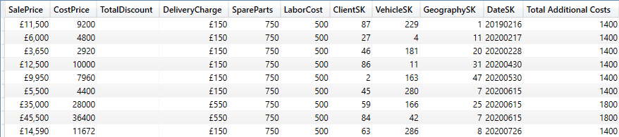
If your requirements are as simple as returning the complete contents of a table from the source Power BI dataset to a paginated report, then you can simply use the EVALUATE keyword, like this:

EVALUATE
FactSales

The output from the sample dataset is as shown below:

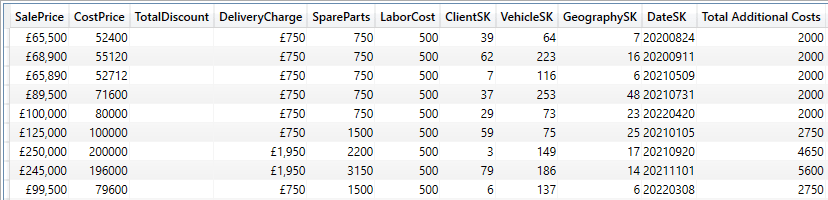
Indeed, this principle can be extended to reduce the output from a single table by enclosing the table to evaluate in a FILTER() function, like this:

EVALUATE
FILTER(
FactSales
,FactSales[CostPrice] > 50000
)

The output (shortened) is as shown in the following image:

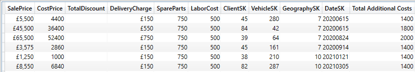
Indeed, you can even filter using values from other tables if you include the RELATED() function inside the FILTER() – much as you would use it when creating calculated columns in a table that need to refer to other tables’ data. You can see this in the following piece of DAX:

EVALUATE
FILTER(
FactSales
,RELATED(DimGeography[CountryName]) = "FRANCE"
)

Sample output is as shown in the following image (where the Geography_SKs only relate to France):

This method means that you can use the full breadth of the data model to filter data even when resorting to the simplest possible DAX.

Note: You need to be aware at this point that you cannot display the filtered field using a simple EVALUATE function. However, you can see the field that you are filtering on if you use SELECTCOLUMNS() –as is explained in a following section.

When using a FILTER() function inside EVALUATE the filtering rules are similar to those described in the previous articles in this series. However, you need to be aware that:

  • Unlike when filtering inside SUMMARIZECOLUMNS(), the table that you are evaluating is, by definition, the filtered object (so there is no need to use VALUES(<tablename>) approach that you used when filtering inside a SUMMARIZECOLUMNS() function).
  • You can only filter on a single column per FILTER() keyword. Consequently multiple filter elements require nested filters – like in this example, where I have added an OR condition for good measure):
EVALUATE
FILTER(
FILTER(
FactSales
,RELATED(DimGeography[CountryName]) = "FRANCE")
,RELATED(DimVehicle[Make]) = "Rolls Royce"
         || RELATED(DimVehicle[Make]) = "Jaguar")

The output (shortened again) is as shown in the following image:

SELECTCOLUMNS() – Used to Return Data from a Single Table

The next DAX table function that delivers non-aggregated output is SELECTCOLUMNS(). This function can be very useful when producing fairly simple lists of fields. After all, this is what paginated reports good at delivering, and may be one of the fundamental reasons that you are using paginated reports rather than Power BI to produce a specific report.

You can use SELECTCOLUMNS() to:

  • Build a custom subset of required columns from a table without any aggregation applied.
  • Change column names.
  • Apply columns of calculations.

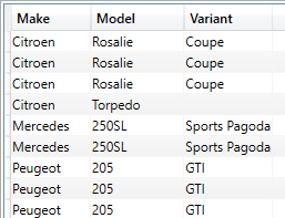
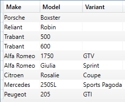
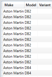
As an example, take a look at the following short piece of DAX, which shows the key attributes of the SELECTCOLUMNS() function:

EVALUATE
SELECTCOLUMNS
(
DimVehicle
,"Make", [Make]
,"Model", [Model]
,"Variant", [ModelVariant]
)

A subset of the output is as shown in the following image (note that there are many records without a model variant, so you will need to scroll to the bottom of the dataset to see the variant detail):

The key points to note are that:

  • The first element of SELECTCOLUMNS() is the table that you want to return data from.
  • All the remaining elements are output name/source column pairs.
  • The column name to use in the output must be supplied, must be in double-quotes, and can contain spaces.
  • You do not have to use fully-qualified field names (table & field) for each output field. The field names themselves must be enclosed in square brackets or double-quotes.
  • SELECTCOLUMNS() performs no aggregation on the source table.

If, for whatever reason, you want to return distinct values using SELECTCOLUMNS(), then you can wrap SELECTCOLUMNS() inside a DISTINCT() function, like this:

EVALUATE
DISTINCT
(
  SELECTCOLUMNS
  (
  DimVehicle
  ,"Make", [Make]
  ,"Model", [Model]
  ,"Variant", [ModelVariant]
  )
)

The output (shortened) is as shown in the following image:

SELECTCOLUMNS() – Used to Return Data from Multiple Tables

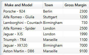
Another possible step when outputting lists is to use SELECTCOLUMNS() to return data from multiple tables in the data model. In this respect, SELECTCOLUMNS() is a bit like adding a calculated column in DAX in Power BI in that you have to tell DAX to traverse the dataset if you want to mix and match columns from multiple tables. You can see this in the following DAX snippet:

EVALUATE
SELECTCOLUMNS
(
FactSales
,"Make and Model", RELATED(DimVehicle[Make]) & " - " &
                   RELATED(DimVehicle[Model])
,"Town", RELATED(DimGeography[Town])
,"Gross Margin", FactSales[SalePrice] - FactSales[CostPrice]
)

The output (shortened) is as shown in the following image:

The points of note at this juncture are:

  • Use RELATED() to traverse the dataset
  • As RELATED() is used, this can mean that only relatively simple data models can be used. Remember, RELATED() follows an existing many-to-one relationship to fetch the value from the specified column in the related table. In other words, if you have a classic star or snowflake schema, then things could work quite easily. The trick may well be to define the fact table as the “core” table as the SELECTCOLUMNS() first parameter, and any dimensional attributes will use RELATED().
  • It is possible to use field names (without qualifying the field name with the table name) only for the fields from the “core” table that is specified as the first element in the SELECTCOLUMNS() function.
  • All fields wrapped in the RELATED() function must be fully qualified (table and field) field names.
  • SELECTCOLUMNS() can also create “calculated columns” in the output as evidenced by the new “Gross Margin” calculation in the DAX above.

I find it useful to think of SELECTCOLUMNS() as something similar to what you can achieve in Power BI Desktop to extend a tabular data subset with merged and calculated columns. It is all about composing and delivering an output dataset from one or more tables in the data model. Also, if you have been using SUMMARIZECOLUMNS() to return data until now, then it is also worth noting that you can add the fields (fields from the core table, fields from related tables and calculations) in any order.

Filtering Output with SELECTCOLUMNS()

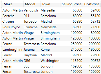
You can easily filter the output from a SELECTCOLUMNS() function. The classic approach is to filter the table that is referred to as the first parameter of SELECTCOLUMNS() – like this

EVALUATE
SELECTCOLUMNS
(
FILTER(FactSales, FactSales[CostPrice] > 50000)
,"Make", RELATED(DimVehicle[Make])
,"Model", RELATED(DimVehicle[Model])
,"Town", RELATED(DimGeography[Town])
,"Selling Price", FactSales[SalePrice]
,FactSales[CostPrice]
)

The output will look something like the shortened snapshot that you can see below:

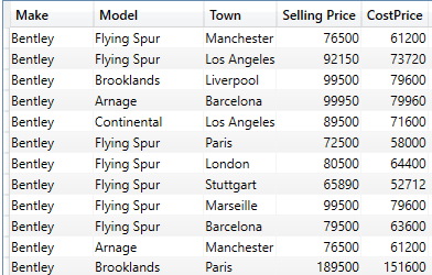
You can, of course, nest logical AND filters by nesting FILTER() functions – like this:

EVALUATE
SELECTCOLUMNS
(
  FILTER
  (
    FILTER
    (
           FactSales, FactSales[CostPrice] > 50000
    )
   ,RELATED(DimVehicle[Make]) = "Bentley"
  )
,"Make", RELATED(DimVehicle[Make])
,"Model", RELATED(DimVehicle[Model])
,"Town", RELATED(DimGeography[Town])
,"Selling Price", FactSales[SalePrice]
, FactSales[CostPrice]
)

A subset of the output is as shown in the following image:

Note that any filters that concern columns not present in the core table must be referred to using RELATED(). Also, you do not, of course, have to display the fields that you are filtering on. I have done this to make the point that the filters are working as expected.

An alternative approach to filtering the data can be to filter the whole output – that is, to wrap the entire SELECTCOLUMNS() function inside a FILTER() function. If you do this, however, the filter can only be applied to a column specified as part of the SELECTCOLUMNS() function. Consequently, this approach can return columns that are not required for the report in the output. An example of this technique is given below:

EVALUATE
FILTER(
       SELECTCOLUMNS
       (
        DimVehicle
        ,"Make", DimVehicle[Make]
        ,"Model", DimVehicle[Model]
        ,"Variant", [ModelVariant]
       )
, ISBLANK([Variant])
)

The output (shortened) is as shown in the following image:

There are a few complexities that it is worth being aware of:

  • You need a clear understanding the data model in order to use the RELATED() function.
  • Measures can be used with SELECTCOLUMNS().
  • There are many subtleties and variations on the theme of filtering data. Fortunately, filtering datasets returned to paginated reports using SELECTCOLUMNS() generally only requires the techniques that you saw in the previous article.

SELECTCOLUMNS() is extremely useful when you want to return simplified list output with a reasonable level of data filtering. The ability to rename columns is also an advantage in certain cases.

ADDCOLUMNS()

Another very useful DAX function that you can use to query a Power BI dataset is ADDCOLUMNS(). This is:

  • Similar to SELECTCOLUMNS() – but it extends a data table rather than starting from scratch with a blank output to which you add further selected columns.
  • Another “Calculated column” approach to extending an existing non-aggregated data table for output to paginated reports.

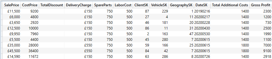
The following DAX sample illustrates how ADDCOLUMNS() can be used:

EVALUATE
ADDCOLUMNS
(
FactSales
,"Gross Profit", FactSales[SalePrice] - FactSales[CostPrice]
)

The output (shortened) is as shown in the following image:

As you can see from the output, this approach returns all the source table elements, plus any others that have been added. If you need the entire table, then this is faster to code. Of course, sending many columns that will never be used in a table across the ether will consume not only bandwidth but also the processing capacity of the Power BI Service, needlessly – and possibly expensively. However, if your data model has tables that lend themselves to being used in their entirety, then ADDCOLUMNS() can be a very useful addition to your paginated report toolkit.

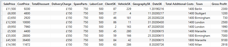
You can, as was the case with SELECTCOLUMNS(), extend the output with fields from other tables using the RELATED() function.

EVALUATE
ADDCOLUMNS
(
FactSales
,"Town", RELATED(DimGeography[Town])
,"Gross Profit", FactSales[SalePrice] - FactSales[CostPrice]
)

The output (shortened) is as shown in the following image:

As was the case with SELECTCOLUMNS(), you can add the fields (fields from the core table, fields from related tables and calculations) in any order. Once again, this presumes a coherent and well thought out data model.

Now that you have seen the non-aggregation DAX table functions, it is time to take a look at two other aggregation functions – SUMMARIZE() and GROUPBY().

SUMMARIZE

SUMMARIZE() is considered by many DAX aficionados as having lost its relevance since SUMMARIZECOLUMNS() was introduced. It is, in many respects, an older, quirky and more verbose version of what is now the standard approach to returning aggregated datasets.

This does not preclude the use of this function. However, as you can see from the code sample below, you have to specify a source table when using SUMMARIZE():
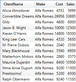
EVALUATE
SUMMARIZE(
FactSales
,DimCLient[ClientName]
,DimVehicle[Make]
,"Cost", SUM(FactSales[CostPrice])
,"Sales", SUM(FactSales[SalePrice])
)
ORDER BY DimCLient[ClientName], DimVehicle[Make]

The output, shown below, is a perfectly valid aggregated table:

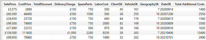
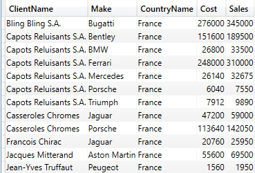
Filtering data using SUMMARIZE() is not difficult, but it does require applying the filter to the table that is used as the source for the SUMMARIZE() function (with all the associated rigmarole of having to use RELATED()) as you can see in the following piece of DAX:

EVALUATE
SUMMARIZE(
FILTER(FactSales, RELATED(DimGeography[CountryName]) = "France")
,DimCLient[ClientName]
,DimVehicle[Make]
,DimGeography[CountryName]
,"Cost", SUM(FactSales[CostPrice])
,"Sales", SUM(FactSales[SalePrice])
)
ORDER BY DimCLient[ClientName], DimVehicle[Make]

You can see the output from this piece of DAX in the following table:

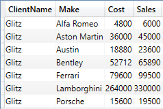
Alternatively, you can wrap the entire SUMMARIZE() function in a CALCULATETABLE() function, like this:

EVALUATE
CALCULATETABLE
(
  SUMMARIZE
  (
  FactSales
  ,DimCLient[ClientName]
  ,DimVehicle[Make]
  ,"Cost", SUM(FactSales[CostPrice])
  ,"Sales", SUM(FactSales[SalePrice])
  )
,DimCLient[ClientName] = "Glitz"
)

The output to this query is shown below:

CALCULATETABLE(), of course, will modify the filter context – whereas FILTER() is an iterator function. For paginated reports, modifying the filter context could be largely irrelevant as long as the paginated report dataset is feeding into a single table or chart in the .rdl file. So, in many cases, CALCULATETABLE() could be a simpler way to filter data. And it opens the path to using modifiers (such as ALL(), ALLEXCEPT() etc) to create more complex filters.

Yet another alternative is to wrap the output from a SUMMARIZE() function in one or more FILTER() functions, as you have seen previously. However, this, once again, necessitates adding the column that you will be filtering on to the output from the SUMMARIZE() function.

So, while it is worth knowing that SUMMARIZE() exists, most people prefer to use SUMMARIZECOLUMNS() unless there is a valid reason for not using the more modern function.

GROUPBY

The final major DAX table function used to return data directly is GROUPBY(). Specifically, if you need nested groupings, then GROUPBY() is particularly useful, as this technique is not possible with SUMMARIZE() or SUMMARIZECOLUMNS().

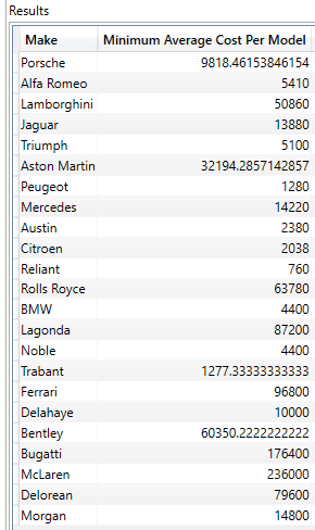
An example of this requirement is finding the lowest average cost price for a car model per make. The following DAX snippet delivers this back to SSRS:

EVALUATE
GROUPBY 
(
  GROUPBY
    (
     FactSales
     ,DimVehicle[Make]
     ,DimVehicle[Model]
     ,"Avg Cost", AVERAGEX(CURRENTGROUP(), FactSales[CostPrice])
     )
,DimVehicle[Make]
,"Minimum Average Cost Per Model", MINX(CURRENTGROUP(), [Avg Cost])
)

The complete output is as shown in the following image:

In this DAX snippet, the inner GROUPBY() finds the average cost for each model per make, and then the outer GROUPBY() returns the maximum model cost per make. Although this approach is generally slower than using SUMMARIZE() or SUMMARIZECOLUMNS() there are challenges – such as this one – that are not possible using other functions.

The main thing to note here is that GROUPBY uses CURRENTGROUP() to provide the row context for the iteration over the virtual table created by the custom grouping. Be warned, however, that GROUPBY() can be slow when applied to large datasets.

Conclusion

As you have learned, there is a small suite of DAX table functions that you can use to return data to paginated reports from a Power BI dataset. A good understanding of the available functions and how they can be used, individually or together, will help you deliver the output you wish to display in your paginated reports. The next article will cover several more DAX table functions.


The post DAX table functions for paginated reports: Part 1 appeared first on Simple Talk.


from Simple Talk https://ift.tt/3fL5OuB
via

When to use CHAR, VARCHAR, or VARCHAR(MAX)

In every database, there are different kinds of data that need to be stored. Some data is strictly numeric, while other data consists of only letters or a combination of letters, numbers, and even special symbols. Whether it is just stored in memory or on disk, each piece of data requires a data type. Picking the correct data type depends on the characteristics of the data being stored. This article explains the differences between CHAR, VARCHAR, and VARCHAR(MAX).

When selecting a data type for a column, you need to think about the characteristics of the data to pick the correct data type. Will each value be the same length, or will the size vary greatly between values? How often will the data change? Will the length of the column change over time? There might also be other factors, like space efficiency and performance, that might drive your decision on a data type.

The CHAR, VARCHAR, and VARCHAR(MAX) data types can store character data. This article will discuss and compare these three different character data types. The information found in this article will help you decide when it is appropriate to use each of these data types.

CHAR the fixed-length character data type

The CHAR data type is a fixed-length data type. It can store characters, numbers, and special characters in strings up to 8000 bytes in size. CHAR data types are best used for storing data that is of a consistent length. For example, two-character State codes in the United States, single-character sex codes, phone numbers, postal codes, etc. A CHAR column would not be a good choice for storing data where the length varies greatly. Columns storing things like addresses or memo fields would not be suitable for a CHAR column data type.

This doesn’t mean a CHAR column can’t contain a value that varies in size. When a CHAR column is populated with strings shorter than the length of the column, spaces will be padded to the right. The number of spaces padded is based on the size of the column less the length of characters being stored. Because CHAR columns are fully populated by adding spaces, when needed, each column uses the same amount of disk space or memory. Trailing spaces also make it a challenge when searching and using CHAR columns. More on this in a moment.

VARCHAR the variable-length character data type

VARCHAR columns, as the name implies, store variable-length data. They can store characters, numbers, and special characters just like a CHAR column and can support strings up to 8000 bytes in size. A variable-length column only takes up the space it needs to store a string of characters, with no spaces added to pad out the column. For this reason, VARCHAR columns are great for storing strings that vary greatly in size.

To support variable-length columns, the length of the data needs to be stored along with the data. Because the length needs to be calculated and used by the database engine when reading and storing variable-length columns, they are considered a little less performant than CHAR columns. However, when you consider they only use the space they need, the savings in disk space alone might offset the performance cost of using a VARCHAR column.

Differences between CHAR and VARCHAR data types

The fundamental difference between CHAR and VARCHAR is that the CHAR data type is fixed in length, while the VARCHAR data type supports variable-length columns of data. But they are also similar. They both can store alphanumeric data. To better understand the differences between these two data types, review the similarities and differences found in Table 1.

Table 1: Differences between CHAR and VARCHAR

CHAR

VARCHAR

Used to store strings of fixed size

Used to store strings of variable length

Can range in size from 1 to 8000 bytes

Can range in size from 1 to 8000 bytes

Uses a fixed amount of storage, based on the size of the column

Use varying amounts of storage space based on the size of the string stored.

Takes up 1 to 4 byte for each character, based on collation setting

Takes up 1 to 4 byte for each character based on collation and requires one or more bytes to store the length of the data

Better performance

Slightly poorer performance because length has to be accounted for.

Pads spaces to the right when storing strings less than the fixed size length

No padding necessary because it is variable in size

What does the “N” mean in CHAR(N) or VARCHAR(N)

The “N” does not mean the maximum number of characters that can be stored in a CHAR or VARCHAR column but instead means the maximum number of bytes a data type will take up. SQL Server has different collations for storing characters. Some character sets, like Latin, store each character in one byte of space. In contrast, other character sets, like the one for Japanese, require multiple bytes to store a character.

CHAR and VARCHAR columns can store up to 8000 bytes. If a single-byte character set is used, up to 8000 characters can be stored in a CHAR or VARCHAR column. If a multi-byte collation is used, the maximum number of characters that a VARCHAR or CHAR can store will be less than 8000. A discussion on collation is outside the scope of this article, but if you want to find out more about single and multi-byte character sets, then check out this documentation.

Truncation error

When a column is defined as a CHAR(N) or VARCHAR(N), the “N” represents the number of bytes that can be stored in the column. When populating a CHAR(N) or VARCHAR(N) column with a character string, a truncation error like shown in Figure 1 might occur.

Figure 1: Truncation error

This error occurs when trying to store a string longer than the maximum length of a CHAR or VARCHAR column. When a truncation error like this occurs, the TSQL code terminates, and any following code will not be executed. This can be demonstrated using the code in Listing 1.

Listing 1: Code to produce truncation error

USE tempdb;
GO
CREATE TABLE MyTable (A VARCHAR(10));
INSERT INTO MyTable VALUES ('This String');
-- Continue on 
SELECT COUNT(*) FROM MyTable;
GO

The code in Listing 1 produced the error in Figure 1 when the INSERT statement is executed. The SELECT statement following the INSERT statement was not executed because of the truncation error. The truncation error and script termination might be exactly the functionality you might want, but there are times when you might not want a truncation error to terminate your code.

Suppose there is a need to migrate data from an old system to a new system. In the old system, there is a table MyOldData that contains data created using the script in Listing 2.

Listing 2: Table in old system

USE tempdb;
GO
CREATE TABLE MyOldData (Name VARCHAR(20), ItemDesc VARCHAR(45));
INSERT INTO MyOldData 
VALUES ('Widget', 'This item does everything you would ever want'), 
       ('Thing A Ma Jig', 'A thing that dances the jig');
GO

The plan is to migrate the data in MyOldData table to a table named MyNewTable, which has a smaller size for the ItemDesc column. The code in Listing 3 is used to create this new table and migrate the data.

Listing 3: Migrating data to a new table

USE tempdb;
GO 
CREATE TABLE MyNewData (Name VARCHAR(20), ItemDesc VARCHAR(40));
INSERT INTO MyNewData SELECT * FROM MyOldData;
SELECT * FROM MyNewData;
GO

When the code in Listing 3 is run, you get a truncation error similar to the error in Figure 1, and no data is migrated.

In order to successfully migrate the data, you need to determine how to deal with the data truncation to make sure all rows migrate across. One method is to truncate the item description using the SUBSTRING function by running the code in Listing 4.

Listing 4: Eliminating truncation error with SUBSTRING

DROP Table MyNewData
GO
USE tempdb;
GO 
CREATE TABLE MyNewData (Name VARCHAR(20), ItemDesc VARCHAR(40));
INSERT INTO MyNewData SELECT Name, substring(ItemDesc,1,40) 
FROM MyOldData;
SELECT * FROM MyNewData;
GO

When running the code in Listing 4, all records are migrated. Those with an ItemDesc longer than 40 will be truncated using the SUBSTRING function, but there is another way.

If you want to avoid the truncation error without writing special code to truncate columns that are too long, you can set the ANSI_WARNINGS setting to off, as done in Listing 5.

Listing 5: Eliminating truncation error by setting ANSI_WARNINGS to off.

DROP Table MyNewData
GO
USE tempdb;
GO 
CREATE TABLE MyNewData (Name VARCHAR(20), ItemDesc VARCHAR(40));
SET ANSI_WARNINGS OFF;
INSERT INTO MyNewData SELECT * FROM MyOldData;
SET ANSI_WARNINGS ON;
SELECT * FROM MyNewData;
GO

By setting the ANSI_WARNINGS off, the SQL Server engine does not follow the ISO standard for some error conditions, one of those being the truncation error condition. When this setting is turned off, SQL Server automatically truncates the source column to fit in target columns without producing an error. Care should be used when turning off ANSI_WARNINGS because other errors might also go unnoticed. Therefore, changing the ANSI_WARNING setting should be used cautiously.

VARCHAR(MAX)

The VARCHAR(MAX) data type is similar to the VARCHAR data type in that it supports variable-length character data. VARCHAR(MAX) is different from VARCHAR because it supports character strings up to 2 GB (2,147,483,647 bytes) in length. You should consider using VARCHAR(MAX) only when each string stored in this data type varies considerably in length, and a value might exceed 8000 bytes in size.

You might be asking yourself, why not use VARCHAR(MAX) all the time, instead of using VARCHAR? You could, but here are a few reasons why you might not want to do that:

VARCHAR(MAX) columns cannot be included as a key column of an index.

VARCHAR(MAX) columns do not allow you to restrict the length of the column.

In order to store large strings, VARCHAR(MAX) columns use LOB_DATA allocation units for large strings. LOB_DATA storage is much slower than using IN_ROW_DATA storage allocation units.

LOB_DATA storage doesn’t support page and row compression.

You might be thinking VARCHAR(MAX) columns will eliminate the truncation error that we saw earlier. That is partially true, provided you don’t try to store a string value longer than 2,147,483,647 bytes. If you do try to store a string that is longer than to 2,147,483,647 bytes in size, you will get the error shown in Figure 2.

Figure 2: Error when a string is longer than 2 GB in size

You should only use VARCHAR(MAX) columns when you know some of the data you are going to store exceed the 8000-byte limit of a VARCHAR(N) column, and all of the data is shorter than the 2 GB limit for the VARCHAR(MAX) column.

Concatenation problems with CHAR Columns

When a CHAR column is not fully populated with a string of characters, the extra unused characters are padded with spaces. When a CHAR column is padding with spaces, it might cause some problems when concatenating CHAR columns together. To better understand this, here are a few examples that use the table created in Listing 6.

Listing 6: Sample Table

USE tempdb;
GO
CREATE TABLE Sample (
ID int identity,
FirstNameChar CHAR(20),
LastNameChar CHAR(20),
FirstNameVarChar VARCHAR(20),
LastNameVarChar VARCHAR(20));
INSERT INTO Sample VALUES ('Greg', 'Larsen', 'Greg', 'Larsen');

The Sample table created in Listing 6 contains 4 columns. The first two columns are defined as CHAR(20) and the second two columns are defined as VARCHAR(20) columns. These columns will be used to store my first and last name.

In order to demonstrate the concatenation problem associated with padded CHAR columns, run the code in Listing 7.

Listing 7: Showing concatenation problem

SELECT FirstNameChar + LastNameChar AS FullNameChar, 
       FirstNameVarChar + LastNameVarChar AS FullNameVarChar FROM Sample;

Report 1 contains the output when Listing 7 is executed

Report 1: Output when code in Listing 7 is run

Image showing what happens when CHAR datatype is used and there are extra spaces between the words.

In Report 1, the FirstNameCHAR column contains several spaces between my first and last name. These spaces came from the spaces that were padded onto the FirstNameCHAR column when it was stored in the CHAR column. The FullNameVARCHAR column does not contain any spaces between first and last name. No spaces are padded when column values are less than the length of the VARCHAR column.

When concatenating CHAR columns, you might need to remove the trailing spaces to get the results you want. One method of eliminating the spaces can be done using the RTRIM function, as shown in Listing 8.

Listing 8: Removing trailing spaces using the RTRIM function

SELECT RTRIM(FirstNameChar) + RTRIM(LastNameChar) AS FullNameChar, 
       FirstNameVarChar + LastNameVarChar AS FullNameVarchar 
FROM Sample;

Output in Report 2 created when Listing 8 is executed is shown below.

Report 2: Output when Listing 8 is run

Image showing results when spaces are removed before concatenation GregLarsen GregLarsen

By using the RTRIM function, all the additional spaces added to the FirstNameCHAR and the LastNameCHAR columns were removed before the concatenation operations were performed.

Problems searching CHAR columns for spaces

Because CHAR columns might be padded with spaces, searching for a space might be problematic.

Suppose you have a table containing phrases, like the one created in Listing 9.

Listing 9: Creating Phrase table

USE tempdb;
GO
CREATE TABLE Phrase (PhraseChar CHAR(100));
INSERT INTO Phrase VALUES ('Worry Less'),
                          ('Oops'),
                          ('Think Twice'),
                          ('Smile');

Some phrases in table Phrase consist of just a single word, while the rest have two words. To search the Phrase table to find all the phrases that contain two words, the code in Listing 10 is used.

Listing 10: Trying to find two-word phrases

SELECT PhraseChar FROM Phrase WHERE PhraseChar like '% %';

The output in Report 3 is produced when Listing 10 is run.

Report 3: Output when Listing 10 is executed

Text Description automatically generated with medium confidence

Why did all the phrases in the Phrase table get returned when only two rows contained 2-word phrases? The search string % % also found the spaces that were padded to the end of the column values. Once again, the RTRIM can be used to make sure the spaces associated with the padding are not included in the search results by running the code in Listing 11.

Listing 11: Removing the trailing spaces

SELECT PhraseChar FROM Phrase
WHERE RTRIM(PhraseChar) like '% %';

I’ll leave it up to you to run the code in Listing 11 to verify if it only finds two-word phrases.

Performance consideration between VARCHAR and CHAR

The amount of work the database engine has to perform to store and retrieve VARCHAR columns is more than it takes for a CHAR column. Every time a VARCHAR column is retrieved, the Database engine has to use the length information stored with the data to retrieve a VARCHAR column value. Using this length information takes extra CPU cycles. Whereas a CHAR column and its fixed length allow SQL Server to more easily chunk through CHAR column based on their fixed-length column definitions.

Disk space is also an issue to consider when dealing with CHAR and VARCHAR columns. Because CHAR columns are fixed-length, they will always take up the same amount of disk space. VARCHAR columns vary in size, so the amount of space needed is based on the size of the strings being storeded instead of the size of the column definition. When a large majority of the values stored in a CHAR column are less than the defined size, then possibly using a VARCHAR column might actually use less disk space. When less disk space is used, less I/O needs to retrieve and store the column value, which means better performance. For these two reasons, choose between CHAR and VARCHAR wisely based on the varying size of the string values being stored.

CHAR, VARCHAR, and VARCHAR(MAX)

CHAR columns are fixed in size, while VARCHAR and VARCHAR(MAX) columns support variable-length data. CHAR columns should be used for columns that vary little in length. String values that vary significantly in length and are no longer than 8,000 bytes should be stored in a VARCHAR column. If you have huge strings (over 8,000 bytes), then VARCHAR(MAX) should be used. In order to store VARCHAR columns, the length information along with the data is stored. Calculating and storing the length value for a VARCHAR column means SQL Server has to do a little more work to store and retrieve VARCHAR columns over CHAR column data types.

The next time you need to decide if a new column should be a CHAR, VARCHAR, or VARCHAR(MAX) column, ask yourself a few questions to determine the appropriate data type. Are all the string values to be stored close to the same size? If the answer is yes, then you should use a CHAR. If strings to be stored vary greatly in size, and values are all less than or equal to 8,000 bytes in size, then use VARCHAR. Otherwise, VARCHAR(MAX) should be used.

If you liked this article, you might also like SQL Server identity column.

The post When to use CHAR, VARCHAR, or VARCHAR(MAX) appeared first on Simple Talk.


from Simple Talk https://ift.tt/3ImGTtx
via

Wednesday, January 19, 2022

Vertipaq optimization and its impact on columnstore compression

Columnstore compression is an impressive array of algorithms that can take large analytic tables and significantly reduce their storage footprint. In doing so, IO is also reduced, and query performance dramatically improved.

This article dives into one aspect of columnstore compression that tends to get buried in all of the hoopla surrounding how awesome columnstore indexes are: Vertipaq optimization. This is a critical component of the columnstore compression process, and understanding how it works can significantly improve the performance of analytic workloads while reducing the computing resources required for the underlying data.

Overview of the columnstore compression process

Columnstore compression can be roughly broken down into three distinct steps:

  1. Encoding
  2. Optimization
  3. Compression

Each of these steps is critical to efficiently storing analytic data, and their order is equally important. Each segment in a columnstore index is compressed separately. This allows different columns of different data types and content to be compressed based on whatever algorithms are best for the values contained within each specific segment.

All compression algorithms discussed in this article are lossless in nature and ultimately rely on exploiting repetition within a data set. The following is a brief review of each compression step and its contribution towards compact OLAP data.

Encoding

The first set of processes used by SQL Server to compress data are transformations known as encoding algorithms. These attempt to restructure data in ways that take up less space. Encoding helps to reduce the footprint of large data types and makes it easier for subsequent compression algorithms to compress effectively. Here are a few examples of common encoding algorithms.

Dictionary encoding

When data values within a segment are a combination of repetitive and wide, dictionary encoding will often be used to “pseudo-normalize” the data prior to further compression. While string data is most often the target of this algorithm, it may also apply to numeric (or other) data types.

In dictionary encoding, each distinct value within a segment is inserted into a dictionary lookup structure and indexed using a numeric key. Each value within the segment is then pointed to the lookup table using its numeric index. For example, consider the following data sample for a column:

Value

Size in Bytes
Mario 5
Sonic the Hedgehog 18
Mario 5
Yoshi 5
Ness 4
Pikachu 7
Sonic the Hedgehog 18
Yoshi 5
Link 4

The values in this column are string-based and contain some repetition. If dictionary encoding were used, an indexed dictionary would be created that looks like this:

ID (Numeric)

Value (String)

0

Link

1

Mario

2

Ness

3

Pikachu

4

Sonic the Hedgehog

5

Yoshi

Once a dictionary is created, the rows within the segment are assigned to their corresponding dictionary lookup, and the index IDs used going forward instead of the explicit string values. The result is a transformation from the initial segment data into a dictionary compressed segment, as shown in this diagram:

In this example, nine string values were replaced with numeric values. When the dictionary index is created, the data type for the ID is chosen based on the number of distinct values. In this case, 3 bits are enough to store all possible values (zero through five). When complete, the size of the original data sample can be compared with the dictionary encoded results. The string data sample contained nine strings totalling 71 bytes if the data type is VARCHAR or 142 bytes if it is NVARCHAR. The dictionary contains six values totaling 43 bytes. The dictionary encoded table contains nine values, each consuming 3 bits, for a total of 27 bits, or 4 bytes, rounding up.

The savings increases as the number of repeated values increase. If this were a typical data sample for a full columnstore segment containing 1,048,576 repetitive string values, then the savings could be quite immense!

Value encoding

Value encoding attempts to shrink the size of data by manipulating how it is stored to use smaller data types. Encoding is accomplished via mathematical transformations to the underlying data and is used exclusively on numeric data types. The easiest way to illustrate this is via an example. The following is a set of integer values:

Value Size in Bits
1700 11
289000 19
500 9
10000 14
1000 10
2000000 21

These values are likely stored in an INT or BIGINT column and therefore consume 4 bytes or 8 bytes each, respectively. The bits are provided as a reference since columnstore compression will use as little space as possible to store values, regardless of data type. Value encoding will attempt to find common divisors for all values in the segment and applying the appropriate exponent to all values to shrink their footprint. For the sample values above, all are divisible by 100, and therefore can be rewritten like this:

Value

Value * 10-2

Size (bits)

1700

17

5

289000

2890

12

500

5

3

10000

100

7

1000

10

4

2000000

20000

15

This transformation divides all values by 100, denoting that the common negative exponent for each value is 10-2. The result of this first transformation is a reduction in storage from 84 bits to 46 bits. Another transformation used in value encoding is to rebase the values using whatever value is closest to zero. This is an additive operation that, in the case of this example, will take the smallest absolute value in the list (five) and subtract it from all values, like this:

Value

Value * 10-2

Value * 10-2 – 5

Size (bits)

1700

17

12

4

289000

2890

2885

12

500

5

0

0

10000

100

95

7

1000

10

5

3

2000000

20000

19995

15

This further decreases storage by another 5 bits. This may seem small, but it does represent an 11% reduction from the previous step and 51% overall compression, which is quite impressive! When this data is stored, it will be maintained alongside the exponent and rebasing value so that decompression can occur quickly by reversing these operations.

Compression

The optimization step is being intentionally skipped (for the moment) to introduce compression. This step uses a variety of compression algorithms that comprise the xVelocity algorithm to reduce the size of segment data as much as possible. While the details of this algorithm are not public, it is safe to make some assumptions about how this data is compressed based on the information that is publicly available. There are multiple algorithms commonly used, including bit-array compression and run-length encoding. Columnstore archive compression implements more aggressive compression techniques and is intended for data that is cool/cold, rather than warm/hot.

The simplest and biggest space-saver regarding columnstore compression is run-length encoding, which takes values that repeat consecutively and compresses them into single entries that signify their value and the number of times it repeats. In analytic data, values often repeat, thus allowing this algorithm to provide significant savings when applied. Consider this example data:


Some values repeat consecutively and can be simplified into a value and magnitude:

This simplification reduces the number of values that need to be stored by three (from twelve to nine). They’d likely also be previously dictionary compressed, further reducing the storage footprint. Note that there are still multiple values that repeat in this list and are stored repeatedly. This is a significant hurdle towards the ability for run-length encoding to effectively compress data. This challenge leads into the headlining topic for this article: Vertipaq Optimization.

Optimization

In rowstore tables, row order is critical to the function of clustered indexes and the performance of typical OLTP queries. A table with a clustered index on an ID column will be ordered on that column so that index seeks on that key can quickly return results. That order is essential for the maintenance of binary-tree indexes and makes perfect sense for common OLTP data scenarios.

Columnstore indexes throw all of that out the window. There is no built-in row order. When building a columnstore index, the data order is determined by however the architect had rows ordered prior to its creation. Azure Synapse Analytics and Parallel Data Warehouse provide syntax for the initial ordering of data within a columnstore index, but once created, maintaining data order is up to whatever processes write data to the index.

This means that once compressed, the order of rows within each rowgroup does not matter. This allows for row order optimization to occur. This is a process that determines an optimal row order based on the order that generates the best compression ratio for the underlying data. The highest compression ratios will typically be those that move as many repeated values into adjacent groupings as possible. This greatly benefits run-length encoding and further enhances the impact of encoding steps taken earlier in the compression process.

Note that a row order is determined for an entire rowgroup, which means that the row order for any one segment may be quite optimal, whereas the order for another segment may be suboptimal. Despite that detail, like values tend to group together across segments, and SQL Server is capable of determining a good row order, even when many different columns are present. Reconsidering the run-length encoding example from the previous section, applying row order optimization to the data would reduce storage further, as shown by this diagram:

Rearranging row order allowed for each of the three pairs of repeated values to be combined further, reducing the row count from nine to six. Note that the count of values for each distinct entry has not changed. Reordering rows, though, allowed for additional values to be combined via run-length encoding.

Vertipaq Optimization is the proprietary process used by Microsoft in compressing analytic data on many of their platforms, including SSAS, PowerPivot, Power BI, and in columnstore indexes. Whenever a rowgroup is created or modified, this optimization will be automatically used whenever possible.

The details as to whether or not a rowgroup has been optimized can be viewed in SQL Server via the system view dm_db_column_store_row_group_physical_stats as a bit. The following query returns this information for each rowgroup within a specific columnstore index:

SELECT
    schemas.name AS schema_name,
    objects.name AS table_name,
    dm_db_column_store_row_group_physical_stats.partition_number,
    dm_db_column_store_row_group_physical_stats.row_group_id,
    dm_db_column_store_row_group_physical_stats.has_vertipaq_optimization
FROM sys.dm_db_column_store_row_group_physical_stats
INNER JOIN sys.objects
ON objects.object_id = 
    dm_db_column_store_row_group_physical_stats.object_id
INNER JOIN sys.schemas
ON schemas.schema_id = objects.schema_id
INNER JOIN sys.indexes
ON indexes.index_id = 
    dm_db_column_store_row_group_physical_stats.index_id
AND indexes.object_id = 
    dm_db_column_store_row_group_physical_stats.object_id
WHERE objects.name = 'Sale'
ORDER BY dm_db_column_store_row_group_physical_stats.row_group_id, 
    dm_db_column_store_row_group_physical_stats.partition_number;

The results provide a row per rowgroup and whether Vertipaq Optimization has been used when segments were compressed within each rowgroup:

For the columnstore index on Fact.Sale, one rowgroup in partition 6 has Vertipaq Optimization, whereas the other three rowgroups in partitions 3, 4, and 5 do not. While this sample columnstore index in WideWorldImportersDW is not very large, it can be used to demonstrate the impact on compression when Vertipaq Optimization is not used. Row count and size can be added to the previous query, like this:

SELECT
    schemas.name AS schema_name,
    objects.name AS table_name,
    dm_db_column_store_row_group_physical_stats.partition_number,
    dm_db_column_store_row_group_physical_stats.row_group_id,
    dm_db_column_store_row_group_physical_stats.has_vertipaq_optimization,
    dm_db_column_store_row_group_physical_stats.total_rows,
    dm_db_column_store_row_group_physical_stats.deleted_rows,
    dm_db_column_store_row_group_physical_stats.size_in_bytes
FROM sys.dm_db_column_store_row_group_physical_stats
INNER JOIN sys.objects
ON objects.object_id = 
    dm_db_column_store_row_group_physical_stats.object_id
INNER JOIN sys.schemas
ON schemas.schema_id = objects.schema_id
INNER JOIN sys.indexes
ON indexes.index_id = 
    dm_db_column_store_row_group_physical_stats.index_id
AND indexes.object_id = 
    dm_db_column_store_row_group_physical_stats.object_id
WHERE objects.name = 'Sale'
ORDER BY dm_db_column_store_row_group_physical_stats.row_group_id, 
    dm_db_column_store_row_group_physical_stats.partition_number;

The results show how many rows there are in each rowgroup and their size:

What happened!? Why do three rowgroups lack Vertipaq Optimization? For a large columnstore index, this could be quite costly! More importantly, what can we do about it!?

When does optimization not occur?

Vertipaq optimization is a resource-intensive step that needs to occur quickly whenever a rowgroup is written to. This not only includes columnstore index creation, but also data loads that INSERT, UPDATE, or DELETE data within rowgroups. Because of this, there are two common scenarios where optimization will not occur:

  • Memory-optimized columnstore indexes
  • Clustered columnstore indexes with non-clustered rowstore indexes when delta store rowgroups are merged into compressed rowgroups.

The primary reason that these index configurations will forgo Vertipaq Optimization is due to the cost associated with rearranging rows in each scenario. Memory-optimized tables are structured as row-based solutions to solve contentious OLTP workloads. Regardless of how a memory-optimized table is indexed (columnstore or rowstore), the underlying data is stored in a row-by-row configuration. This differs from disk-based columnstore indexes, which are physically stored by column rather than row.

This is not to say that memory-optimized columnstore indexes are not valuable, but they will not benefit from Vertipaq Optimization when used. If real-time operational analytics are required from a memory-optimized table, consider the fact that compression ratios may not be as impressive for a memory-optimized columnstore index as they would be for its disk-based counterpart and budget memory appropriately based on that knowledge.

When a clustered columnstore index has non-clustered rowstore indexes added to it, a row mapping must be maintained between the non-clustered and clustered indexes. This is analogous to how nodes in a non-clustered rowstore index contain a copy of the clustered primary key that allow for fast writes or key lookups between the indexes, when needed. For Vertipaq Optimization to work in this scenario would require the row mapping between each non-clustered rowstore index and the clustered columnstore index to be updated whenever the optimization process was applied. This would be quite expensive (aka: SLOW!), and as such, the process is skipped in these scenarios.

While this may seem like a cautionary tale as to why non-clustered rowstore indexes should not be used in conjunction with clustered columnstore indexes, there are ways to mitigate this problem and minimize the impact of it at little cost to the SQL Server that hosts this data.

Steps to resolve unoptimized rowgroups

The primary reason that Vertipaq Optimization is not applied to rowgroups is because non-clustered rowstore indexes were present on the columnstore index when data was written to it. A clustered columnstore index may be built with non-clustered rowstore indexes present, and existing data will be optimized, but additional data that is written later may not be. Despite that situation, optimization can still occur. The following are some strategies for tackling this problem, both pre-emptively and after the fact.

Partitioning

Tables with columnstore indexes can be partitioned just like any other table in SQL Server. Rowgroups do not span partitions, and each partition will have its own unique set of rowgroups. If the partition scheme organizes data based on active versus inactive data (a time-based dimension), then indexing strategies and maintenance can vary from partition to partition. This means that:

  • Older partitions might not need as many (or any) non-clustered rowstore indexes.
  • Older data may never change. If so, it can be subject to a one-time rebuild/cleanup process, after which it will remain optimal indefinitely.
  • If a columnstore index is memory-optimized, then maybe older data that is rarely subject to busy OLTP querying can be separated into disk-based tables/partitions/indexes and not maintained in-memory.

For a large columnstore index, consider partitioning it. The benefits are huge and the drawbacks minimal. Ensure that each partition has enough rows to comprise many rowgroups so that rowgroups are not inadvertently undersized.

Initial build considerations

When creating a columnstore index for the first time and populating it with data, forgo the non-clustered indexes until after the initial build is complete. This will not only allow optimization to occur, but it will speed up the data load as SQL Server does not need to write to both clustered and non-clustered indexes while loading data.

Non-clustered indexes can be created after all data has been inserted, preserving its optimal compression along the way.

Columnstore index rebuilds

While SQL Server will not automatically apply Vertipaq Optimization to newly inserted data in clustered columnstore indexes that have non-clustered rowstore indexes present, re-creating the index will resolve the problem. Note that when performing an index rebuild on the columnstore index, optimization will not necessarily be applied, but it also will not be removed.

This is a helpful key in understanding what the has_vertipaq_optimization bit means as it applies to data that is inserted in the future. Since columnstore indexes have no built-in data order, existing data may or may not be optimized. Future index rebuilds will not take optimized data and “de-optimize” it. Therefore, once data is pristine, it will remain so unless a more disruptive process changes it (such as the use of a clustered rowstore index).

This can be demonstrated with Fact.Sale, for which three of four rowgroups do not have Vertipaq Optimization applied to their compression. The following T-SQL executes a rebuild against the columnstore index:

ALTER INDEX CCX_Fact_Sale ON Fact.Sale REBUILD WITH (ONLINE = ON);

Once complete, checking metadata reveals that no rowgroups have Vertipaq Optimization enabled:

The has_vertipaq_optimization bit is now set to zero, and nothing else has changed. Rebuilding the index did not provide any benefit regarding optimization. With the non-clustered indexes present, getting Vertipaq Optimization applied will require dropping and recreating the columnstore index the old-fashioned way:

DROP INDEX CCX_Fact_Sale ON Fact.Sale;
CREATE CLUSTERED COLUMNSTORE INDEX CCX_Fact_Sale ON Fact.Sale WITH (MAXDOP = 1);

I get

Note that not only is Vertipaq Optimization enabled, but the space consumed by each rowgroup has decreased. The rowgroup that was already optimized has not changed, but the other three have been shrunk from a total of 5,035,816 bytes to 3,346,304. This is about a 34% savings, which underscores the significance of Vertipaq Optimization and how it can greatly improve columnstore compression ratios.

There is an important cautionary lesson here: Limit non-clustered rowstore indexes on clustered columnstore indexes. It is very unlikely that a real-world table needs this many foreign key indexes and including them wastes space and resources. Test queries without supporting indexes first and verify if they are needed or not. If the table is truly analytic in nature, then a well-ordered columnstore index should be able to service most (or all) of the OLAP queries issued against it. If the table serves a mixed workload, consider which is predominant, the OLTP queries or the OLAP queries. If transactional queries dominate, then consider using a clustered rowstore index with a non-clustered columnstore index on the appropriate columns.

Once the rowgroups are optimized, keep in mind that inserting or merging new data into them will result in has_vertipaq_optmization to be set to 0. This can be simulated locally with a REBUILD operation. Note that when data is optimized and has_vertipaq_optimization is later set to zero for a rowgroup, the existing data remains optimized.

For example, consider the similar rowgroup metadata below:

While has_vertipaq_optimization is now shown as zero for all rebuilt partitions, it has had no impact on the size of those rowgroups and will only impact data written in the future. Therefore, there is value in only issuing index maintenance against active partitions that need it. Older data that has already had Vertipaq Optimization applied will not benefit from further rebuild processes unless the data is modified somehow before that maintenance.

Index maintenance strategy

The impact of non-clustered indexes on a clustered columnstore index leads to the need to target index maintenance to the data that requires it most. In most typical data warehouse scenarios, data is written once (or multiple times over a short span of time) and then not altered again. In this situation, it is possible to save the expensive index drop/add or index rebuilds to when the data is no longer hot. This will minimize disruption while ensuring that data at rest is as compact as possible. It will also ensure that infrequent (but resource-hungry) long-term analytics can run as quickly and efficiently as possible. Similarly, read-only data needs only to be targeted by index maintenance one time so long as it is not written again.

Validating Vertipaq optimization

Using simplified versions of queries already introduced in this article, it becomes easy to check for any columnstore index rowgroups that do not have Vertipaq Optimization. The following query returns filtered details about any columnstore rowgroups that are not optimized:

SELECT
        schemas.name AS schema_name,
        objects.name AS table_name,
        indexes.name AS index_name,
        dm_db_column_store_row_group_physical_stats.partition_number,
        dm_db_column_store_row_group_physical_stats.row_group_id,
        dm_db_column_store_row_group_physical_stats.total_rows,
        dm_db_column_store_row_group_physical_stats.deleted_rows,
        dm_db_column_store_row_group_physical_stats.size_in_bytes
FROM sys.dm_db_column_store_row_group_physical_stats
INNER JOIN sys.objects
ON objects.object_id = 
    dm_db_column_store_row_group_physical_stats.object_id
INNER JOIN sys.schemas
ON schemas.schema_id = objects.schema_id
INNER JOIN sys.indexes
ON indexes.index_id = 
    dm_db_column_store_row_group_physical_stats.index_id
AND indexes.object_id = 
    dm_db_column_store_row_group_physical_stats.object_id
WHERE dm_db_column_store_row_group_physical_stats.has_vertipaq_optimization = 0
ORDER BY schemas.name, objects.name, indexes.name, 
    dm_db_column_store_row_group_physical_stats.row_group_id, 
    dm_db_column_store_row_group_physical_stats.partition_number;

The results show again the four rowgroups from Fact.Sale that were discussed above:

Using this information, an architect or operator can decide how (or if) to take any further actions with index maintenance. Some thoughts on how to proceed given this data:

If rowgroups contain data that is no longer hot, then indexes can easily be dropped and recreated. If the data is heavily used, then an online rebuild could be used to help improve index structure, with a drop/recreate saved for a time when maintenance operations are allowed. Keep in mind that the need to fix unoptimized data should be rare and will often be a one-time operation for analytic data as it is rarely the subject of disruptive update operations. Once a rowgroup is full and optimized, then it will remain optimal indefinitely, even if the has_vertipaq_optimization bit is flipped to zero. Only a significant change to the table’s structure would change that.

If a rowgroup is relatively small and lacks optimization, then dropping an index on a large table to fix that small rowgroup is likely not a good use of resources. Employ index maintenance tactically and only when there is a meaningful benefit to be gained. Generally speaking, optimization will improve compression ratios by at least 25%, though I have personally seen it go as high as 60%. The more repetitive the data, the better the improvement.

Because analytic data is written on more structured schedules by well-defined processes, the need to validate optimization is unlikely to be daily, or even weekly. Consider this as an infrequent check to ensure that storage and IO are not being wasted in large amounts. The accumulated bloat of poorly compressed data will not be seen in a few days but will be realized either when a table is first populated or over time as more data is added.

Conclusion

Optimization is an important step in the columnstore compression algorithm that can greatly reduce storage footprint and improve IO. SQL Server will utilize Vertipaq Optimization whenever possible, but under some circumstances will not. When unable to be used, it is up to us to identify when and why it was skipped and determine the simplest way to proceed.

For a large columnstore index, Vertipaq Optimization can provide significant savings at little cost to an organization. It’s free and easy to use, and all that is needed is knowledge of its existence and how to take advantage of it. Enjoy!

If you liked this article, you might also like Hands-On with Columnstore Indexes: Part 1 Architecture.

The post Vertipaq optimization and its impact on columnstore compression appeared first on Simple Talk.


from Simple Talk https://ift.tt/3GMVUo0
via

Saturday, January 15, 2022

Transformations by the Oracle Optimizer

It’s common knowledge that when you write an SQL statement, you’re describing to the database what you want but not how to get it. It shouldn’t come as a surprise, then, that in all but the simplest cases, the statement that Oracle optimizes isn’t necessarily the statement that you wrote. Putting it another way, Oracle will probably transform your statement into a logically equivalent statement before applying the arithmetic it uses to pick an execution path.

If you want to become skilled in troubleshooting badly performing SQL, it’s important to be able to recognize what transformations have been applied, what transformations haven’t been applied when they could have been, and how to force (or block) the transformations you think will have the greatest impact.

In this article, we’re going to examine one of the oldest and most frequently occurring transformations that the Optimizer considers: unnesting subqueries.

The Optimizer’s wish-list

The “query block” is the starting point for understanding the optimizer’s methods and reading execution plans. Whatever you’ve done in your query, no matter how complex and messy it is, the optimizer would like to transform it into an equivalent query of the form:

select  {list of columns}
from    {list of “tables”}
where   list of simple join and filter predicates}

Optionally your query may have group by, having, and order by clauses as well as any of the various “post-processing” features of newer versions of Oracle, but the core task for the optimizer is to find a path that acquires the raw data in the shortest possible time. The bulk of the optimizer’s processing is focused on “what do you want” (select), “where is it” (from), “how do I connect the pieces” (where). This simple structure is the “query block”, and most of the arithmetic the optimizer does is about calculating the cost of executing each individual query block once.

Some queries, of course, cannot be reduced to such a simple structure – which is why I’ve put “tables” in quote marks and used the word “simple” in the description of predicates. In this context, a “table” could be a “non-mergeable view”, which would be isolated and handled as the result set from a separately optimized query block. If the best that Oracle can do to transform your query still leaves some subqueries in the where clause or select list, then those subqueries would also be isolated and handled as separately optimized query blocks.

When you’re trying to solve a problem with badly performing SQL, it’s extremely useful to identify the individual query blocks from your original query in the final execution plan. Your performance problem may have come from how Oracle has decided to “stitch together” the separate query blocks that it has generated while constructing the final plan.

Case study

Here’s an example of a query that starts life with two query blocks. Note the qb_name() hint that I’ve used to give explicit names to the query blocks; if I hadn’t done this, Oracle would have used the generated names sel$1 and sel$2 for the main and subq query blocks respectively.

select  /*+ qb_name(main) */
        *
from    t1
where   owner = 'OUTLN'
and     object_name in (
                select  /*+ qb_name(subq) */
                       object_name
                from   t2
                where  object_type = 'TABLE'
        )
;

I’ve created both t1 and t2 using selects on the view all_objects so that the column names (and possible data patterns) look familiar and meaningful, and I’ll be using Oracle 12.2.0.1 to produce execution plans as that’s still very commonly in use and things haven’t changed significantly in versions up to the latest release of 19c.

There are several possible plans for this query, depending on how my CTAS filtered or scaled up the original content of all_objects, what indexes I’ve added, and whether I’ve added or removed any not null declarations. I’ll start with the execution plan I get when I add the hint /*+ no_query_transformation */ to the text:

explain plan for 
select  /*+ qb_name(main) no_query_transformation */
        *
from    t1
where   owner = 'sys'
and     object_name in (
                select  /*+ qb_name(subq) */
                       object_name
                from   t2
                where  object_type = 'TABLE'
        )
;
select * from table(dbms_xplan.display(format=>'alias -bytes'));

The plan returned looks like this:

I’ve used explain plan here so that you can see the complete Predicate Information. If I had executed the query and pulled the plan from memory with a call to dbms_xplan.display_cursor(), the predicate information for operation 1 would have read: “1 – filter( IS NOT NULL)”.Since there are no bind variables (and no risk of side-effects due to mismatched character sets), it’s safe to assume that explain plan will produce the correct plan.

There are a few points to pick up on this query and plan:

Even though I have instructed the optimizer to do “no query transformations,” you can see from the Predicate Information for operation 1 that my non-correlated IN subquery has turned into a correlated EXISTS subquery where the correlating object_name has been supplied as a bind variable (:B1). There’s no conflict here between my hint and the optimizer’s transformation – this is an example of a “heuristic” transformation (i.e., the optimizer’s going to do it because there’s a rule to say it can), and the hint relates only to cost-based transformations.

The “alias” information that I requested in my call to dbms_xplan.display() results in the Query Block Name / Object Alias section of the plan being reported. This section allows you to see that the plan is made up of the two query blocks (main and subq) that I had named in the original text. You can also see that t1 and t1_i1 appearing in the body of the plan correspond to the t1 that appeared in the main query block (t1@main), and the t2/t2_i1 corresponds to t2 in the subq query block (t2@subq). This is a trivial observation in this case, but if, for example, you are troubleshooting a long, messy query against Oracle’s General Ledger schema, it’s very helpful to be able to identify where in the query each of the many references to a frequently used GLCC originated.

If you examine the basic shape of this plan, you will see that the main query block has been executed as an index range scan based on the predicate owner = ‘OUTLN’. The subq query block has been executed as an index range scan based on the predicate object_name = {bind variable}. Oracle has then stitched these two query blocks together through a filter operation. For each row returned by the main query block, the filter operation executes the subq query block to see if it can find a matching object_name that is also of type TABLE.

Finally, a comment on Cost: if all you can see is the execution plan, it’s easy to be misled by rounding effects and hidden details of the optimizer allowing for “self-induced caching,” etc. In this case, the base cost of 2 for each execution of the subquery is reduced to 1 in the assumption that the index root block will be cached, and a quick check of the CBO’s trace file (10053 trace) shows that the 1 is actually closer to 1.003 (and the 84 for the t1 access is actually 84.32). Since the optimizer has an estimate of 3,125 rows for the number of rows it will initially fetch from t1 before filtering the total predicted cost of 3219 is approximately: 84.32+ 3125 * 1.003. Realistically, of course, you might expect there to be much more data caching with a hugely reduced I/O load; especially in this case where the total size of the t2 table was only 13 blocks, so a calculation that produced a cost estimate equivalent to more than 3,000 physical read requests for repeated execution of the subquery is clearly inappropriate. Furthermore, the optimizer doesn’t attempt to allow for a feature known as scalar subquery caching so the arithmetic is based on the assumption that the t2 subquery will be executed for each row found in t1.

Here is the section from the CBO’s trace file:

Variations on a theme

The optimizer transformed an IN subquery to an EXISTS subquery. If the value of the object_name in a row from t1 is of interest if it appears in a list of values, then it’s sensible to check by finding that value in the list. If there are duplicates in the list, stop looking after finding the first match. That’s effectively the method of the FILTER operation in the initial plan, but there is an alternative; if the data sets happen to have the right pattern and volume, Oracle could go through virtually the same motions but use a semi_join, which means “for each row in t1 find the first matching row in t2. The plan would be like the following:

The semi-join was actually the strategy that the optimizer chose for my original data set when I allowed cost-based transformations to take place, but it used a hash join rather than a nested loop join. Since t2 was the smaller row source, Oracle also “swapped sides” to get to a hash join that was both “semi” and “right”:

But there’s more

The volumes of data involved might mean it’s a good idea to adopt a completely different strategy – and this is where unnesting becomes apparent. If the volume of data from t1 is so small that you only have to run the check a few times, then an existence test could be a very good idea (especially if there’s an index that supports a very efficient check). If the volume of data from t1 is large or there’s no efficient path into the t2 table to do the check, then it might be better to create a list of the distinct values (of object_name) in t2 and use that list to drive a join into t1. Here’s one example of how the plan could change:

The plan now has a new object at operation 2, a (non-mergeable) view called vw_nso_1 that is recognizably something holding the distinct (hash unique) values of t2.object_name. The number of such values is quite small (only 36 estimated), so the optimizer might have used a nested loop join to collect related rows from t1, but the arithmetic has pushed it into using the “brute force” method of finding all the t1 rows of type TABLE and then doing a hash join.

It’s important to get into the habit of using the alias format option when the shape of the plan doesn’t match the pattern you were expecting to see. In this case, you can see from the Query Block Name information that the final plan consists of two new query blocks: sel$aa0d0e02 and sel$a93afaed. The first query block describes how Oracle will produce a “table” representing the list of distinct object names, and the second query block is a simple join of two “tables” with a hash join. Note how the Object Alias information tells you that the view vw_nso_1 originated in the query block sel$a93afaed.

Side Note: A generated query block name is a hash value generated from the names of the query blocks that were used to produce the new query block, and the hashing function is deterministic.

In effect, the original query has been transformed into the equivalent:

select
        t1.*
from    (
        select
                distinct object_name 
        from    t2 
        where   object_type=’TABLE’
        ) vw_nso_1,
        t1 
where   t1.owner=’OUTLN’ 
and     t1.object_name = vw_nso_1.object_name
/

Whenever you see a view in the plan with a name like vw_nso_{number}, it’s an indication that the optimizer has transformed an IN subquery into an inline view in this way. Interestingly, if you manually rewrite a query to change an IN subquery to an EXISTS subquery, you may find that you get precisely the same plan but with a view named vw_sq_{number}.

And even this strategy could be subject to further transformation if the data pattern warranted it. In my test case, the optimizer does a “distinct aggregation” on a number of small rows before joining to another table to produce much longer rows, which means the aggregation step can be quite efficient. But what if there were a large number of rows to aggregate in t2, and what if the rows were close to being unique and were quite long rows – the aggregation step could require a lot of work for very little benefit. If the join to t1 then eliminated a lot of (aggregated) t2 data and the t1 rows in the select list were quite short, it might be more efficient to join t1 and t2 to eliminate lots of long rows before aggregating to eliminate the duplicates, producing a plan like the following:

As you can see, the optimizer has produced a hash join between t1 and t2 before eliminating duplicates with a “hash unique” operation. This is a little more subtle than it looks because if you tried to write a statement to do this, you could easily make an error that eliminated some rows that should have been kept – an error best explained by examining the approximate equivalent of the statement that Oracle has actually optimized:

select  
        {list of t1 columns}
from    (
        select 
                distinct
                t2.object_name  t2_object_name,
                t1.rowid _owed,
                t1.*
        from
                t2,
                t1
        where
                t1.owner = ‘OUTLN’
        and     t2.object_name = t1.object_name
        and     t2.object_type = ‘TABLE’
        ) vm_nwvw_2
;

Notice the appearance of t1.rowid in the inline view; that’s the critical bit that protects Oracle from producing the wrong results. Since the join is on object_name (which is not unique in the view all_objects that I created my tables from), there could be two rows in t1 and two in t2 all holding the same object_name, with the effect that a simple join would produce four rows.

The final result set should hold two rows (corresponding to the initial two rows in t1), but if the optimizer didn’t include the t1 rowid in the select list before using the distinct operator, those four rows would aggregate down to a single row. The optimizer sometimes has to do some very sophisticated (or possibly incomprehensible) work to produce a correctly transformed statement – which is why the documentation sometimes lists restrictions to new transformations: the more subtle bits of code that would guarantee correct results for particular cases don’t always appear in the first release of a new transformation.

You’ll notice that the generated view name, in this case, takes the form vm_nwvw_{number} Most of the generated view names start with vw_ this one may be the one special case. The view shows one of the effects of “Complex View Merging” – hence the vm, perhaps – where Oracle changes “aggregate then join” into “join then aggregate”, which happens quite often as a step following subquery unnesting.

Summary

If you write a query containing subqueries, whether in the select list or (more commonly) in the where clause, the optimizer will often consider unnesting as many subqueries as possible. This generally means restructuring your subquery into an inline view that can go into the from clause and be joined to other tables in the from clause.

The names of such inline views are typically of the form vw_nso_{number} or vw_sq_{number}.

After unnesting a subquery, Oracle may apply further transformations that make the inline view “disappear” – turning into a join, or semi-join, or (an example we have not examined) an anti-join. Alternatively, the inline view may also be subject to complex view merging, which may introduce a new view with a name of the form vm_nwvw_{number} but may result in the complete disappearance of any view operation.

I haven’t covered the topic of how Oracle can handle joins to or from an unnested view if it turns out to be non-mergeable, and I haven’t said anything about the difference between IN and NOT IN subqueries. These are topics for another article.

Finally, I opened the article with a discussion of the “query block” and its importance to the optimizer. Whenever you write a query, it is a good idea to give every query block its own query block name using the qb_name() hint. When you need to examine an execution plan, it is then a good idea to add the alias format option to the call to dbms_xplan so that you can find your original query blocks in the final plan, see which parts of the plan are query blocks create by optimizer transformation, and see the boundaries where the optimizer has “stitched together” separate query blocks.

Footnote

If you’ve been examining these execution plans in detail, you will have noticed that all five plans look as if they’ve been produced from exactly the same tables – even though my notes were about how different plans for the same query could appear thanks to different patterns in the data. To demonstrate the different plans, I used a minimum number of hints to override the optimizer’s choices. Ultimately, when the optimizer has made a mistake in its choice of transformation, you do need to know how to recognize and control transformations, and you may have to attach hints to your production code.

I’ve often warned people against hinting because of the difficulty of doing it correctly, but hints aimed at query blocks (the level where the transformation choices come into play) are significantly safer than using “micro-management” hints at the object level.

Although I had to use “micro-management” (object-level) hints to switch between the nested loop join and the hash join in the section “Variations on a Theme,” all the other examples made use of query block hints, namely: merge/no_merge, unnest/no_unnest, or semijoin/no_semijoin.


If you liked this article, you might also like Index Costing Threat

The post Transformations by the Oracle Optimizer appeared first on Simple Talk.


from Simple Talk https://ift.tt/3I3ryOv
via